for GODE Review

Import

import numpy as np
import matplotlib.pyplot as plt
import matplotlib
import pandas as pd
import random

import warnings
warnings.simplefilter("ignore", np.ComplexWarning)
from haversine import haversine
from IPython.display import HTML
import plotly.graph_objects as go
import copy 

import tqdm
from rpy2.robjects.packages import importr
from rpy2.robjects.vectors import FloatVector 

from pygsp import graphs, filters, plotting, utils

from sklearn.metrics import confusion_matrix
from sklearn.metrics import precision_score, recall_score, f1_score, accuracy_score

from sklearn.neighbors import LocalOutlierFactor
from pyod.models.knn import KNN
from pyod.models.cblof import CBLOF
from sklearn import svm
from pyod.models.mcd import MCD
from pyod.models.feature_bagging import FeatureBagging
from pyod.models.abod import ABOD
from alibi_detect.od import IForest
from pyod.models.hbos import HBOS
from pyod.models.sos import SOS
from pyod.models.so_gaal import SO_GAAL
from pyod.models.mo_gaal import MO_GAAL
from pyod.models.lscp import LSCP
from pyod.models.lof import LOF
from pyod.models.ocsvm import OCSVM
from sklearn.svm import OneClassSVM

2024-08-12 19:09:35.601442: I tensorflow/core/util/port.cc:110] oneDNN custom operations are on. You may see slightly different numerical results due to floating-point round-off errors from different computation orders. To turn them off, set the environment variable `TF_ENABLE_ONEDNN_OPTS=0`.
2024-08-12 19:09:35.625187: I tensorflow/tsl/cuda/cudart_stub.cc:28] Could not find cuda drivers on your machine, GPU will not be used.
2024-08-12 19:09:35.843821: I tensorflow/tsl/cuda/cudart_stub.cc:28] Could not find cuda drivers on your machine, GPU will not be used.
2024-08-12 19:09:35.845812: I tensorflow/core/platform/cpu_feature_guard.cc:182] This TensorFlow binary is optimized to use available CPU instructions in performance-critical operations.
To enable the following instructions: AVX2 AVX512F AVX512_VNNI FMA, in other operations, rebuild TensorFlow with the appropriate compiler flags.
2024-08-12 19:09:36.595858: W tensorflow/compiler/tf2tensorrt/utils/py_utils.cc:38] TF-TRT Warning: Could not find TensorRT
/home/csy/anaconda3/envs/pygsp/lib/python3.10/site-packages/tqdm/auto.py:21: TqdmWarning: IProgress not found. Please update jupyter and ipywidgets. See https://ipywidgets.readthedocs.io/en/stable/user_install.html
  from .autonotebook import tqdm as notebook_tqdm

Simulation

Class Code

class Conf_matrx:
    def __init__(self,original,compare):
        self.original = original
        self.compare = compare
    def conf(self,name):
        self.conf_matrix = confusion_matrix(self.original, self.compare)
        
        fig, ax = plt.subplots(figsize=(5, 5))
        ax.matshow(self.conf_matrix, cmap=plt.cm.Oranges, alpha=0.3)
        for i in range(self.conf_matrix.shape[0]):
            for j in range(self.conf_matrix.shape[1]):
                ax.text(x=j, y=i,s=self.conf_matrix[i, j], va='center', ha='center', size='xx-large')
        plt.xlabel('Predictions', fontsize=18)
        plt.ylabel('Actuals', fontsize=18)
        plt.title('Confusion Matrix', fontsize=18)
        plt.show()
        
        self.acc = accuracy_score(self.original, self.compare)
        self.pre = precision_score(self.original, self.compare)
        self.rec = recall_score(self.original, self.compare)
        self.f1 = f1_score(self.original, self.compare)
        
        print('Accuracy: %.3f' % self.acc)
        print('Precision: %.3f' % self.pre)
        print('Recall: %.3f' % self.rec)
        print('F1 Score: %.3f' % self.f1)

class Linear:
    def __init__(self,df):
        self.df = df
        self.y = df.y.to_numpy()
        self.x = df.x.to_numpy()
        self.n = len(self.y)
        self.W = w
    def _eigen(self):
        d= self.W.sum(axis=1)
        D= np.diag(d)
        self.L = np.diag(1/np.sqrt(d)) @ (D-self.W) @ np.diag(1/np.sqrt(d))
        self.lamb, self.Psi = np.linalg.eigh(self.L)
        self.Lamb = np.diag(self.lamb)      
    def fit(self,sd=20): # fit with ebayesthresh
        self._eigen()
        self.ybar = self.Psi.T @ self.y # fbar := graph fourier transform of f
        self.power = self.ybar**2 
        ebayesthresh = importr('EbayesThresh').ebayesthresh
        self.power_threshed=np.array(ebayesthresh(FloatVector(self.ybar**2),sd=sd))
        self.ybar_threshed = np.where(self.power_threshed>0,self.ybar,0)
        self.yhat = self.Psi@self.ybar_threshed
        self.df = self.df.assign(yHat = self.yhat)
        self.df = self.df.assign(Residual = self.df.y- self.df.yHat)

class Orbit:
    def __init__(self,df):
        self.df = df 
        self.f = df.f.to_numpy()
        self.x = df.x.to_numpy()
        self.y = df.y.to_numpy()
        self.n = len(self.f)
        self.theta= None
    def get_distance(self):
        self.D = np.zeros([self.n,self.n])
        locations = np.stack([self.x, self.y],axis=1)
        for i in tqdm.tqdm(range(self.n)):
            for j in range(i,self.n):
                self.D[i,j]=np.linalg.norm(locations[i]-locations[j])
        self.D = self.D + self.D.T
    def get_weightmatrix(self,theta=1,beta=0.5,kappa=4000):
        self.theta = theta
        dist = np.where(self.D < kappa,self.D,0)
        self.W = np.exp(-(dist/self.theta)**2)
    def _eigen(self):
        d= self.W.sum(axis=1)
        D= np.diag(d)
        self.L = np.diag(1/np.sqrt(d)) @ (D-self.W) @ np.diag(1/np.sqrt(d))
        self.lamb, self.Psi = np.linalg.eigh(self.L)
        self.Lamb = np.diag(self.lamb)       
    def fit(self,sd=5,ref=20): # fit with ebayesthresh
        self._eigen()
        self.fbar = self.Psi.T @ self.f # fbar := graph fourier transform of f
        self.power = self.fbar**2 
        ebayesthresh = importr('EbayesThresh').ebayesthresh
        self.power_threshed=np.array(ebayesthresh(FloatVector(self.fbar**2),sd=sd))
        self.fbar_threshed = np.where(self.power_threshed>0,self.fbar,0)
        self.fhat = self.Psi@self.fbar_threshed
        self.df = self.df.assign(fHat = self.fhat)
        self.df = self.df.assign(Residual = self.df.f- self.df.fHat)
        self.bottom = np.zeros_like(self.f)
        self.width=0.05
        self.depth=0.05

class BUNNY:
    def __init__(self,df):
        self.df = df 
        self.f = df.f.to_numpy()
        self.z = df.z.to_numpy()
        self.x = df.x.to_numpy()
        self.y = df.y.to_numpy()
        self.noise = df.noise.to_numpy()
        self.fnoise = self.f + self.noise
        self.W = _W
        self.n = len(self.f)
        self.theta= None
    def _eigen(self):
        d= self.W.sum(axis=1)
        D= np.diag(d)
        self.L = np.diag(1/np.sqrt(d)) @ (D-self.W) @ np.diag(1/np.sqrt(d))
        self.lamb, self.Psi = np.linalg.eigh(self.L)
        self.Lamb = np.diag(self.lamb)       
    def fit(self,sd=5,ref=6): # fit with ebayesthresh
        self._eigen()
        self.fbar = self.Psi.T @ self.fnoise # fbar := graph fourier transform of f
        self.power = self.fbar**2 
        ebayesthresh = importr('EbayesThresh').ebayesthresh
        self.power_threshed=np.array(ebayesthresh(FloatVector(self.fbar**2),sd=sd))
        self.fbar_threshed = np.where(self.power_threshed>0,self.fbar,0)
        self.fhat = self.Psi@self.fbar_threshed
        self.df = self.df.assign(fnoise = self.fnoise)
        self.df = self.df.assign(fHat = self.fhat)
        self.df = self.df.assign(Residual = self.df.f + self.df.noise - self.df.fHat)
        self.bottom = np.zeros_like(self.f)
        self.width=0.05
        self.depth=0.05

5

Linear

np.random.seed(6)
epsilon = np.around(np.random.normal(size=1000),15)
signal = np.random.choice(np.concatenate((np.random.uniform(-7, -5, 25).round(15), np.random.uniform(5, 7, 25).round(15), np.repeat(0, 950))), 1000)
eta = signal + epsilon

outlier_true_one_1 = signal.copy()

outlier_true_one_1 = list(map(lambda x: -1 if x!=0 else 1,outlier_true_one_1))

x_1 = np.linspace(0,2,1000)
y1_1 = 5 * x_1
y_1 = y1_1 + eta # eta = signal + epsilon

_df=pd.DataFrame({'x':x_1, 'y':y_1})

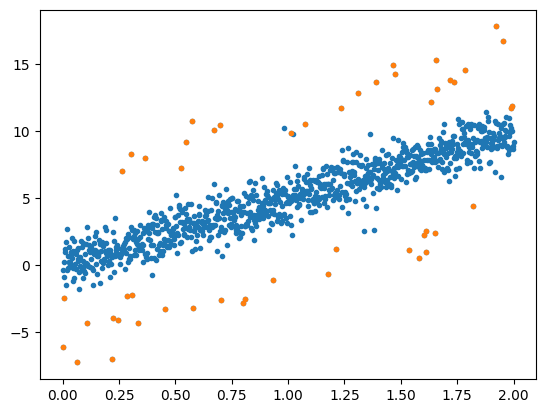
plt.plot(_df.x,_df.y,'.')

KNN

from pyod.models.knn import KNN

np.random.seed(77)
clf = KNN(contamination=0.05)
clf.fit(_df[['x', 'y']])
_df['knn_Clf'] = clf.labels_

outlier_KNN_one = list(clf.labels_)

outlier_KNN_one = list(map(lambda x: 1 if x==0  else -1,outlier_KNN_one))

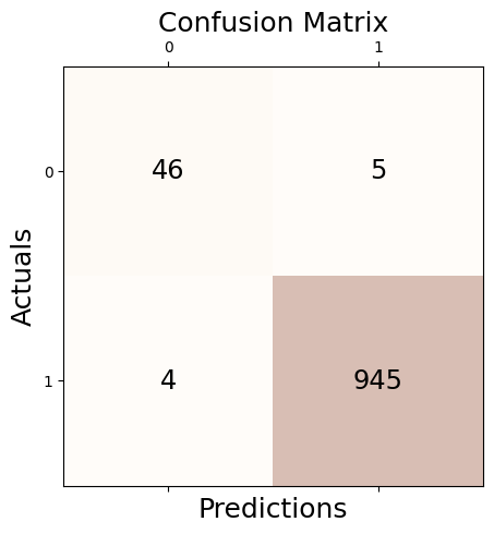
_conf = Conf_matrx(outlier_true_one_1,outlier_KNN_one)

_conf.conf("kNN (Ramaswamy et al., 2000)")

Accuracy: 0.991
Precision: 0.995
Recall: 0.996
F1 Score: 0.995

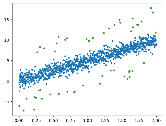
plt.plot(_df.x,_df.y,'.')
plt.plot(_df.query('knn_Clf==1').x,_df.query('knn_Clf==1').y,'.')

MCD(Minimum covaraicen determinant)

clf = MCD(contamination=0.05, random_state = 77)
clf.fit(_df[['x', 'y']])
_df['MCD_clf'] = clf.labels_

outlier_MCD_one = list(clf.labels_)

outlier_MCD_one = list(map(lambda x: 1 if x==0  else -1,outlier_MCD_one))

_conf = Conf_matrx(outlier_true_one_1,outlier_MCD_one)

_conf.conf("MCD (Hardin and Rocke, 2004)")

Accuracy: 0.999
Precision: 0.999
Recall: 1.000
F1 Score: 0.999

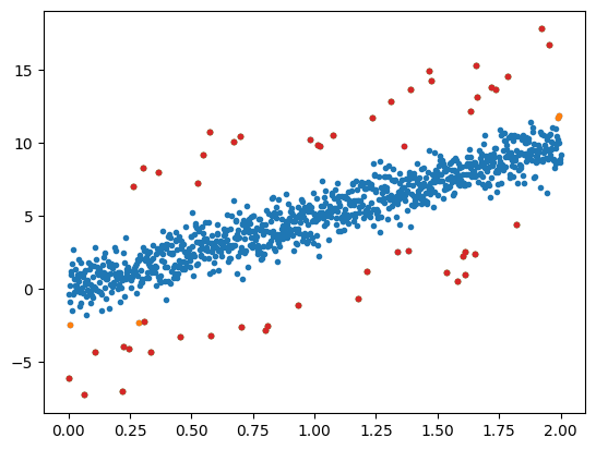
plt.plot(_df.x,_df.y,'.')
plt.plot(_df.query('knn_Clf==1').x,_df.query('knn_Clf==1').y,'.')
plt.plot(_df.query('MCD_clf==1').x,_df.query('MCD_clf==1').y,'.')

_df['outlier'] = outlier_true_one_1

plt.plot(_df.x,_df.y,'.')
plt.plot(_df.query('knn_Clf==1').x,_df.query('knn_Clf==1').y,'.')
plt.plot(_df.query('MCD_clf==1').x,_df.query('MCD_clf==1').y,'.')
plt.plot(_df.query('outlier==-1').x,_df.query('outlier==-1').y,'.')

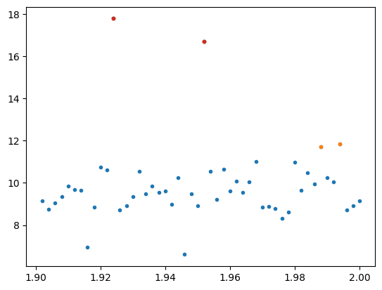
knn default k=5

plt.plot(_df.x[950:],_df.y[950:],'.')
plt.plot(_df[950:].query('knn_Clf==1').x,_df[950:].query('knn_Clf==1').y,'.')
plt.plot(_df[950:].query('MCD_clf==1').x,_df[950:].query('MCD_clf==1').y,'.')
plt.plot(_df[950:].query('outlier==-1').x,_df[950:].query('outlier==-1').y,'.')

_df.query('outlier==-1 and knn_Clf!=1')

	x	y	knn_Clf	MCD_clf	outlier
491	0.982983	10.268781	0	1	-1
510	1.021021	9.762030	0	1	-1
668	1.337337	2.531418	0	1	-1
681	1.363363	9.811717	0	0	-1
690	1.381381	2.661736	0	1	-1

_df.query('outlier==1 and knn_Clf!=0')

	x	y	knn_Clf	MCD_clf	outlier
4	0.008008	-2.446741	1	0	1
142	0.284284	-2.268814	1	0	1
993	1.987988	11.702880	1	0	1
996	1.993994	11.861119	1	0	1

_df.query('outlier==-1 and MCD_clf!=1')

	x	y	knn_Clf	MCD_clf	outlier
681	1.363363	9.811717	0	0	-1

_df.query('outlier==1 and MCD_clf!=0')

	x	y	knn_Clf	MCD_clf	outlier

6

np.random.seed(777)
epsilon = np.around(np.random.normal(size=1000),15)
signal = np.random.choice(np.concatenate((np.random.uniform(-4, -1, 25).round(15), np.random.uniform(1, 4, 25).round(15), np.repeat(0, 950))), 1000)
eta = signal + epsilon
pi=np.pi
n=1000
ang=np.linspace(-pi,pi-2*pi/n,n)
r=5+np.cos(np.linspace(0,12*pi,n))
vx=r*np.cos(ang)
vy=r*np.sin(ang)
f1=10*np.sin(np.linspace(0,6*pi,n))
f = f1 + eta
_df = pd.DataFrame({'x' : vx, 'y' : vy, 'f' : f,'f1':f1})
outlier_true_orbit = signal.copy()
outlier_true_orbit = list(map(lambda x: 1 if x!=0 else 0,outlier_true_orbit))
index_of_trueoutlier_bool = signal!=0

_Orbit = Orbit(_df)
_Orbit.get_distance()

100%|██████████| 1000/1000 [00:01<00:00, 760.96it/s]

_Orbit.D[_Orbit.D>0].mean()

6.453496488349201

_Orbit.D.mean()

6.4470429918608545

np.sort(_Orbit.D.reshape(-1))

array([ 0.      ,  0.      ,  0.      , ..., 11.999822, 11.999822,
       11.999822])

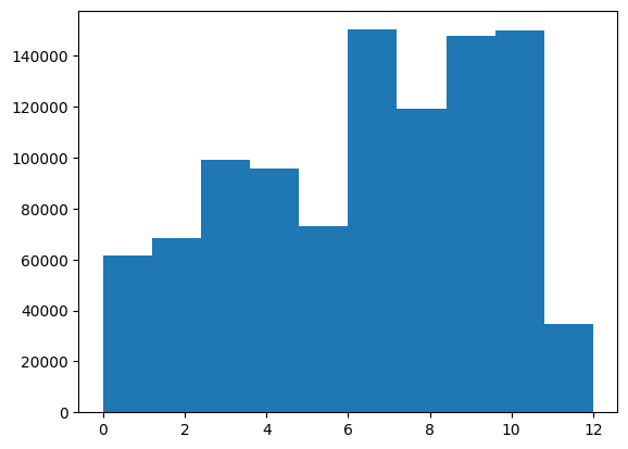
plt.hist(_Orbit.D[_Orbit.D<2500])

(array([ 61680.,  68300.,  99308.,  95596.,  72980., 150314., 119168.,
        147688., 150170.,  34796.]),
 array([ 0.       ,  1.1999822,  2.3999644,  3.5999466,  4.7999288,
         5.999911 ,  7.1998932,  8.3998754,  9.5998576, 10.7998398,
        11.999822 ]),
 <BarContainer object of 10 artists>)

_Orbit.get_weightmatrix(theta=(_Orbit.D[_Orbit.D>0].mean()),kappa=2500) 
# _Orbit.fit(sd=15)

_Orbit.D.max()

11.999821996562474

np.where(_Orbit.D < 2500,_Orbit.D,0)

array([[0.        , 0.03770354, 0.07543358, ..., 0.11310466, 0.07539662,
        0.03769905],
       [0.03770354, 0.        , 0.03774828, ..., 0.15076287, 0.11308224,
        0.07539662],
       [0.07543358, 0.03774828, 0.        , ..., 0.18839838, 0.15076287,
        0.11310466],
       ...,
       [0.11310466, 0.15076287, 0.18839838, ..., 0.        , 0.03774828,
        0.07543358],
       [0.07539662, 0.11308224, 0.15076287, ..., 0.03774828, 0.        ,
        0.03770354],
       [0.03769905, 0.07539662, 0.11310466, ..., 0.07543358, 0.03770354,
        0.        ]])

epsilon = np.around(np.random.normal(size=1000),15)
signal = np.random.choice(np.concatenate((np.random.uniform(-7, -5, 25).round(15), np.random.uniform(5, 7, 25).round(15), np.repeat(0, 950))), 1000)
eta = signal + epsilon

eta.mean()

-0.04969203925183714

7

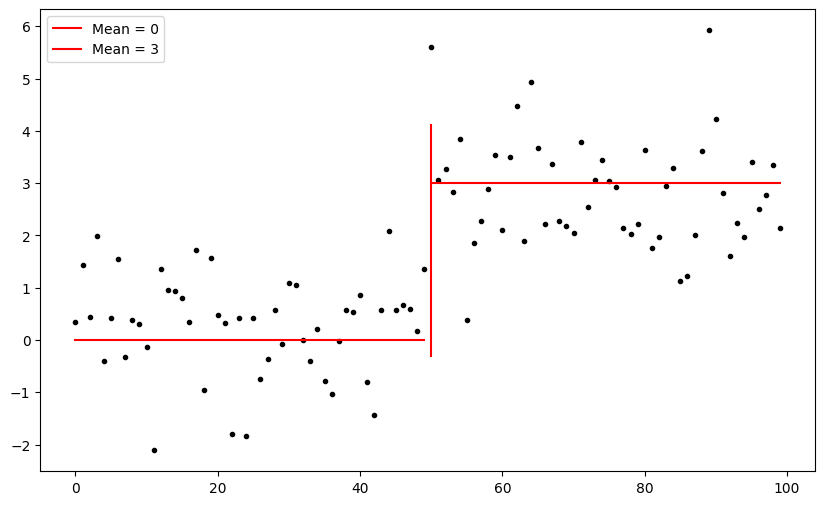
data1 = np.random.normal(size=50)
data2 = np.random.normal(size=50) + 3
x = np.array(range(0,100))

fig,ax = plt.subplots(figsize=(10,6))
ax.plot(x[:50], data1, '.', color='black')
ax.plot(x[50:], data2, '.', color='black')

ax.plot(x[:50], [0]*50, '-', color='red', label = 'Mean = 0')
ax.plot(x[50:], [3]*50, '-', color='red', label = 'Mean = 3')
ax.axvline(x=50, ymin=2/8, ymax=6/8, color='red', linestyle='-')
ax.legend()

p-value: 0.5827

num_nodes = 100

# 자기 자신만 연결된 상태의 가중치 행렬 초기화
weight_matrix = np.eye(num_nodes)  # 대각선 요소만 1, 나머지 요소는 0인 단위 행렬 생성

# 가중치 행렬 출력
print(weight_matrix)

[[1. 0. 0. ... 0. 0. 0.]
 [0. 1. 0. ... 0. 0. 0.]
 [0. 0. 1. ... 0. 0. 0.]
 ...
 [0. 0. 0. ... 1. 0. 0.]
 [0. 0. 0. ... 0. 1. 0.]
 [0. 0. 0. ... 0. 0. 1.]]

연결이 다 끊어진 상태

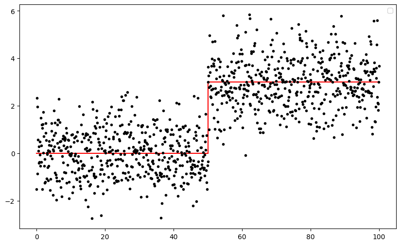
x1 = np.linspace(0, 50, 500)
y1 = np.zeros_like(x1)

x2 = np.linspace(50, 50, 500)
y2 = np.linspace(0, 3, 500) 

x3 = np.linspace(50, 100, 500)
y3 = np.ones_like(x3) * 3

xx = np.concatenate((x1, x3))
yy = np.concatenate((y1, y3))

fig,ax = plt.subplots(figsize=(10,6))

ax.plot(x1, y1, '-', color='red')
ax.plot(x3, y3, '-', color='red')
ax.plot(x2, y2, '-',color='red')
ax.plot(np.concatenate((x1, x3)), np.concatenate((y1 +  np.random.normal(size=500), y3 +  np.random.normal(size=500))),'.', color='black')
ax.legend()
fig.savefig('weakly stationary example_240624.pdf',format='pdf')

adf_result = adfuller(np.concatenate((np.random.normal(size=50) + 3, np.random.normal(size=50))))
print("p-value:", round(adf_result[1],4))

No artists with labels found to put in legend.  Note that artists whose label start with an underscore are ignored when legend() is called with no argument.

p-value: 0.781

8

\(\mathbb{E} \bigg[ \big({\bf S}^a{\bf y}\big)\Big(\big({\bf S}^H)^b {\bf y}\Big)^H \bigg]=\mathbb{E}\bigg[\big({\bf S}^{a+c}{\bf y}\big)\Big(\big({\bf S}^H\big)^{b-c}{\bf y} \Big)^H \bigg]\)

A = np.array([
    [0, 1, 0, 0, 0, 0, 0],
    [0, 0, 1, 0, 0, 0, 0],
    [0, 0, 0, 1, 0, 0, 0],
    [0, 0, 0, 0, 1, 0, 0],
    [0, 0, 0, 0, 0, 1, 0],
    [0, 0, 0, 0, 0, 0, 1],
    [1, 0, 0, 0, 0, 0, 0]
])
S = A
S

array([[0, 1, 0, 0, 0, 0, 0],
       [0, 0, 1, 0, 0, 0, 0],
       [0, 0, 0, 1, 0, 0, 0],
       [0, 0, 0, 0, 1, 0, 0],
       [0, 0, 0, 0, 0, 1, 0],
       [0, 0, 0, 0, 0, 0, 1],
       [1, 0, 0, 0, 0, 0, 0]])

y = np.array(np.random.normal(loc=0, scale=1, size=7)).reshape(7,1)
np.mean(y)

0.8065480054630054

y

array([[0.21544054],
       [0.04388057],
       [0.40884195],
       [2.09964748],
       [0.93647026],
       [0.41473195],
       [1.52682329]])

\(a = 2, b = 2, c = 1\)

np.mean((S @ S @ y) @ (np.conjugate(np.conjugate(S) @ np.conjugate(S) @ y)).T)

0.6505196851163523

np.mean((S @ S @ S @ y) @ np.conjugate(np.conjugate(S) @ y ).T)

0.6505196851163523

S @ S @ S

array([[0, 0, 0, 1, 0, 0, 0],
       [0, 0, 0, 0, 1, 0, 0],
       [0, 0, 0, 0, 0, 1, 0],
       [0, 0, 0, 0, 0, 0, 1],
       [1, 0, 0, 0, 0, 0, 0],
       [0, 1, 0, 0, 0, 0, 0],
       [0, 0, 1, 0, 0, 0, 0]])

S

array([[0, 1, 0, 0, 0, 0, 0],
       [0, 0, 1, 0, 0, 0, 0],
       [0, 0, 0, 1, 0, 0, 0],
       [0, 0, 0, 0, 1, 0, 0],
       [0, 0, 0, 0, 0, 1, 0],
       [0, 0, 0, 0, 0, 0, 1],
       [1, 0, 0, 0, 0, 0, 0]])

np.conjugate(S) == S

array([[ True,  True,  True,  True,  True,  True,  True],
       [ True,  True,  True,  True,  True,  True,  True],
       [ True,  True,  True,  True,  True,  True,  True],
       [ True,  True,  True,  True,  True,  True,  True],
       [ True,  True,  True,  True,  True,  True,  True],
       [ True,  True,  True,  True,  True,  True,  True],
       [ True,  True,  True,  True,  True,  True,  True]])

np.conjugate(y) == y

array([[ True],
       [ True],
       [ True],
       [ True],
       [ True],
       [ True],
       [ True]])

S @ S @ y

array([[0.40884195],
       [2.09964748],
       [0.93647026],
       [0.41473195],
       [1.52682329],
       [0.21544054],
       [0.04388057]])

y

array([[0.21544054],
       [0.04388057],
       [0.40884195],
       [2.09964748],
       [0.93647026],
       [0.41473195],
       [1.52682329]])