import pandas as pd
import matplotlib.pyplot as plt
import seaborn as sns1
df_pharmacy_sales = pd.read_csv("../../../delete/Demo Pharmacy Sales Data.csv")
df_pharmacy_sales| Date Sold | Med_name | Med_class | Quantity Sold | Price | |
|---|---|---|---|---|---|
| 0 | 2021-05-07 | Clotrimazole Topical Cream (2%) | Antifungal | 66 | 86.9 |
| 1 | 2021-08-09 | Alprostadil Urethral Suppository (125 mcg) | Prostaglandin E1 Analog | 15 | 22.9 |
| 2 | 2021-06-15 | Methyltestosterone Tablet (10 mg) | Androgen Hormone | 5 | 5.9 |
| 3 | 2021-02-19 | Buspirone Tablet (5 mg) | Anxiolytic | 89 | 55.7 |
| 4 | 2022-09-24 | Hydrocodone/Acetaminophen Tablet (5/325 mg) | Opioid Analgesic/Analgesic Combination | 79 | 0.7 |
| ... | ... | ... | ... | ... | ... |
| 999995 | 2020-11-29 | Alprostadil Urethral Suppository (125 mcg) | Prostaglandin E1 Analog | 34 | 58.0 |
| 999996 | 2021-03-30 | Fenoprofen Tablet (600 mg) | Nonsteroidal Anti-Inflammatory Drug | 12 | 98.3 |
| 999997 | 2020-04-17 | Doxazosin Tablet (1 mg) | Alpha-Blocker | 83 | 10.3 |
| 999998 | 2021-12-08 | Flumazenil Injection (0.1 mg/mL) | Benzodiazepine Antagonist | 1 | 23.9 |
| 999999 | 2022-08-16 | Prednisolone Tablet (5 mg) | Corticosteroid | 44 | 54.5 |
1000000 rows × 5 columns
기본 정보 보기
df_pharmacy_sales.info()<class 'pandas.core.frame.DataFrame'>
RangeIndex: 1000000 entries, 0 to 999999
Data columns (total 5 columns):
# Column Non-Null Count Dtype
--- ------ -------------- -----
0 Date Sold 1000000 non-null object
1 Med_name 1000000 non-null object
2 Med_class 1000000 non-null object
3 Quantity Sold 1000000 non-null int64
4 Price 1000000 non-null float64
dtypes: float64(1), int64(1), object(3)
memory usage: 38.1+ MB이 중 QUantity Sold랑 Price 만 숫자형인 것을 확인할 수 있음
summary_stats = df_pharmacy_sales[['Quantity Sold','Price']].describe()
summary_stats| Quantity Sold | Price | |
|---|---|---|
| count | 1000000.000000 | 1000000.000000 |
| mean | 50.524566 | 50.024411 |
| std | 28.847235 | 28.872706 |
| min | 1.000000 | 0.100000 |
| 25% | 26.000000 | 25.000000 |
| 50% | 51.000000 | 50.000000 |
| 75% | 75.000000 | 75.100000 |
| max | 100.000000 | 100.000000 |
summary 보면 위와 같음
df_pharmacy_sales['Quantity Sold'].plot.hist(bins=30,edgecolor='k')
plt.title("Histogram of Quantity Sold")
plt.show()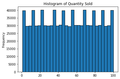
bin 을 어떻게 설정하느냐에 따라 약 판매량 데이터를 다르게 볼 수 있을듯
plt.figure(figsize=(12,4))
plt.subplot(1,2,1)
df_pharmacy_sales['Quantity Sold'].plot.hist(bins=20,edgecolor='k')
plt.title("Histogram of Quantity Sold")

plt.subplot(1,2,2)
df_pharmacy_sales['Price'].plot.hist(bins=20,edgecolor='k')
plt.title("Histogram of Price")

plt.show()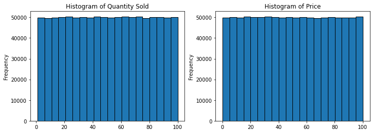
팔린 개수랑 가격이랑 어떻게 범위가 같지..
plt.figure(figsize=(12,4))
plt.subplot(1,2,1)
sns.histplot(df_pharmacy_sales['Quantity Sold'],bins=20,kde=True,color='blue')
plt.title("Histogram of Quantity Sold")

plt.subplot(1,2,2)
sns.histplot(df_pharmacy_sales['Price'],bins=20,kde=True,color='pink')
plt.title("Histogram of Price")

plt.show()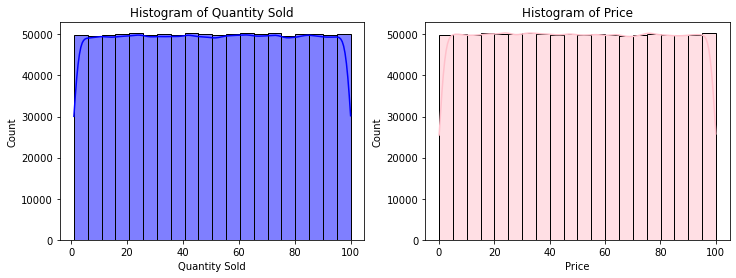
seaborn을 사용해서 데이터를 그려보면 위와 같은데
plot 그리는 방법은 다양하니 참고
2
import pandas as pd
import matplotlib.pyplot as plt
import seaborn as sns
from wordcloud import WordCloud
df_pharmacy_sales = pd.read_csv("../../../delete/Demo Pharmacy Sales Data.csv")
df_pharmacy_sales.head()| Date Sold | Med_name | Med_class | Quantity Sold | Price | |
|---|---|---|---|---|---|
| 0 | 2021-05-07 | Clotrimazole Topical Cream (2%) | Antifungal | 66 | 86.9 |
| 1 | 2021-08-09 | Alprostadil Urethral Suppository (125 mcg) | Prostaglandin E1 Analog | 15 | 22.9 |
| 2 | 2021-06-15 | Methyltestosterone Tablet (10 mg) | Androgen Hormone | 5 | 5.9 |
| 3 | 2021-02-19 | Buspirone Tablet (5 mg) | Anxiolytic | 89 | 55.7 |
| 4 | 2022-09-24 | Hydrocodone/Acetaminophen Tablet (5/325 mg) | Opioid Analgesic/Analgesic Combination | 79 | 0.7 |
단어 시각화를 위해 WordCloud를 쓸거임
df_pharmacy_sales['Med_name'].value_counts()Tretinoin Topical Cream (0.025%) 15027
Ketoconazole Topical Cream (2%) 11008
Adapalene/Benzoyl Peroxide Topical Gel (0.1/2.5%) 10097
Triamcinolone Topical Ointment (0.1%) 10083
Clobetasol Topical Cream (0.05%) 9984
...
Guanfacine Tablet (2 mg) 939
Olopatadine Nasal Spray (665 mcg/spray) 938
Methylphenidate Tablet (10 mg) 938
Lithium Carbonate Capsule (300 mg) 920
Clindamycin Topical Lotion (1%) 917
Name: Med_name, Length: 279, dtype: int64Med_name의 summary는 위와 같음
len(df_pharmacy_sales.query('Med_name=="Guanfacine Tablet (2 mg)"'))939df_pharmacy_sales['Med_class'].value_counts() Nonsteroidal Anti-Inflammatory Drug 82146
Phosphodiesterase Type 5 Inhibitor 56294
Alpha-Blocker 52208
Anticonvulsant 49766
Beta-Blocker 40673
...
Norepinephrine Reuptake Inhibitor 995
Melatonin Receptor Agonist 983
Cardiac Glycoside 981
Anticholinergic/Short-Acting Beta-2 Agonist Combination 977
Mood Stabilizer 920
Name: Med_class, Length: 87, dtype: int64Med_class의 summary는 위와 같음
top_number = 20top_classes = df_pharmacy_sales['Med_class'].value_counts().nlargest(top_number).index
top_classesIndex([' Nonsteroidal Anti-Inflammatory Drug',
' Phosphodiesterase Type 5 Inhibitor', ' Alpha-Blocker',
' Anticonvulsant', ' Beta-Blocker', ' Antifungal', ' Corticosteroid',
' Benzodiazepine', ' Low-Potency Corticosteroid',
' High-Potency Corticosteroid', ' Opioid Analgesic', ' Antibiotic',
' Inhaled Corticosteroid', ' 5-Alpha Reductase Inhibitor', ' Analgesic',
' Prostaglandin E1 Analog', ' Retinoid', ' Sympathomimetic',
' Vasodilator', ' Alpha-2 Agonist'],
dtype='object')df_top_med_classes = df_pharmacy_sales[df_pharmacy_sales['Med_class'].isin(top_classes)]
df_top_med_classes| Date Sold | Med_name | Med_class | Quantity Sold | Price | |
|---|---|---|---|---|---|
| 0 | 2021-05-07 | Clotrimazole Topical Cream (2%) | Antifungal | 66 | 86.9 |
| 1 | 2021-08-09 | Alprostadil Urethral Suppository (125 mcg) | Prostaglandin E1 Analog | 15 | 22.9 |
| 6 | 2018-10-22 | Norepinephrine Injection (2 mg/mL) | Sympathomimetic | 96 | 80.6 |
| 8 | 2022-05-19 | Rofecoxib Tablet (25 mg) | Nonsteroidal Anti-Inflammatory Drug | 32 | 21.2 |
| 9 | 2019-07-21 | Fluticasone Inhaler (50 mcg/actuation) | Inhaled Corticosteroid | 71 | 9.6 |
| ... | ... | ... | ... | ... | ... |
| 999992 | 2018-10-31 | Carbamazepine Tablet (200 mg) | Anticonvulsant | 92 | 73.3 |
| 999995 | 2020-11-29 | Alprostadil Urethral Suppository (125 mcg) | Prostaglandin E1 Analog | 34 | 58.0 |
| 999996 | 2021-03-30 | Fenoprofen Tablet (600 mg) | Nonsteroidal Anti-Inflammatory Drug | 12 | 98.3 |
| 999997 | 2020-04-17 | Doxazosin Tablet (1 mg) | Alpha-Blocker | 83 | 10.3 |
| 999999 | 2022-08-16 | Prednisolone Tablet (5 mg) | Corticosteroid | 44 | 54.5 |
661970 rows × 5 columns
상위 20개만 살펴보고자 할때
df_top_med_classes = df_top_med_classes.groupby('Med_class')['Quantity Sold'].sum().reset_index()
df_top_med_classes| Med_class | Quantity Sold | |
|---|---|---|
| 0 | 5-Alpha Reductase Inhibitor | 1101549 |
| 1 | Alpha-2 Agonist | 802378 |
| 2 | Alpha-Blocker | 2625280 |
| 3 | Analgesic | 1061008 |
| 4 | Antibiotic | 1259910 |
| 5 | Anticonvulsant | 2514863 |
| 6 | Antifungal | 1819102 |
| 7 | Benzodiazepine | 1705063 |
| 8 | Beta-Blocker | 2062362 |
| 9 | Corticosteroid | 1776749 |
| 10 | High-Potency Corticosteroid | 1509454 |
| 11 | Inhaled Corticosteroid | 1112097 |
| 12 | Low-Potency Corticosteroid | 1519123 |
| 13 | Nonsteroidal Anti-Inflammatory Drug | 4153538 |
| 14 | Opioid Analgesic | 1514248 |
| 15 | Phosphodiesterase Type 5 Inhibitor | 2838613 |
| 16 | Prostaglandin E1 Analog | 1060112 |
| 17 | Retinoid | 1019449 |
| 18 | Sympathomimetic | 1005189 |
| 19 | Vasodilator | 973025 |
type(df_top_med_classes.groupby('Med_class')['Quantity Sold'].sum())pandas.core.series.Seriesreset_index하기 전
type(df_top_med_classes)pandas.core.frame.DataFramereset_index 후
df_top_med_classes = df_top_med_classes.sort_values(by='Quantity Sold')
df_top_med_classes| Med_class | Quantity Sold | |
|---|---|---|
| 1 | Alpha-2 Agonist | 802378 |
| 19 | Vasodilator | 973025 |
| 18 | Sympathomimetic | 1005189 |
| 17 | Retinoid | 1019449 |
| 16 | Prostaglandin E1 Analog | 1060112 |
| 3 | Analgesic | 1061008 |
| 0 | 5-Alpha Reductase Inhibitor | 1101549 |
| 11 | Inhaled Corticosteroid | 1112097 |
| 4 | Antibiotic | 1259910 |
| 10 | High-Potency Corticosteroid | 1509454 |
| 14 | Opioid Analgesic | 1514248 |
| 12 | Low-Potency Corticosteroid | 1519123 |
| 7 | Benzodiazepine | 1705063 |
| 9 | Corticosteroid | 1776749 |
| 6 | Antifungal | 1819102 |
| 8 | Beta-Blocker | 2062362 |
| 5 | Anticonvulsant | 2514863 |
| 2 | Alpha-Blocker | 2625280 |
| 15 | Phosphodiesterase Type 5 Inhibitor | 2838613 |
| 13 | Nonsteroidal Anti-Inflammatory Drug | 4153538 |
4
plt.barh(df_top_med_classes['Med_class'],df_top_med_classes['Quantity Sold'])
plt.title(f'Top {top_number} Medication Classes by Quantity Sold')
plt.xlabel("Quantity Sold")
plt.ylabel("Medication Class")
plt.show()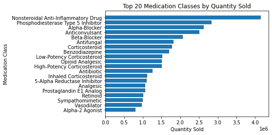
med_classes = df_pharmacy_sales['Med_class'].str.cat(sep='')
wordcloud = WordCloud(width=800,height=400).generate(med_classes)
plt.figure(figsize=(14,7))
plt.imshow(wordcloud,interpolation='bilinear')
plt.show()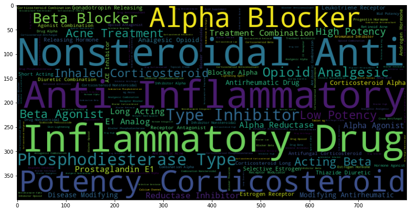
med_names = df_pharmacy_sales['Med_name'].str.cat(sep='')
wordcloud = WordCloud(width=800,height=400).generate(med_names)
plt.figure(figsize=(10,5))
plt.imshow(wordcloud,interpolation='bilinear')
plt.show()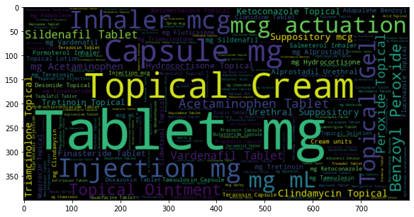
import pandas as pd
import matplotlib.pyplot as plt
import prophet
from prophet import Prophet
df_pharmacy_sales = pd.read_csv("../../../delete/Demo Pharmacy Sales Data.csv")
df_pharmacy_sales| Date Sold | Med_name | Med_class | Quantity Sold | Price | |
|---|---|---|---|---|---|
| 0 | 2021-05-07 | Clotrimazole Topical Cream (2%) | Antifungal | 66 | 86.9 |
| 1 | 2021-08-09 | Alprostadil Urethral Suppository (125 mcg) | Prostaglandin E1 Analog | 15 | 22.9 |
| 2 | 2021-06-15 | Methyltestosterone Tablet (10 mg) | Androgen Hormone | 5 | 5.9 |
| 3 | 2021-02-19 | Buspirone Tablet (5 mg) | Anxiolytic | 89 | 55.7 |
| 4 | 2022-09-24 | Hydrocodone/Acetaminophen Tablet (5/325 mg) | Opioid Analgesic/Analgesic Combination | 79 | 0.7 |
| ... | ... | ... | ... | ... | ... |
| 999995 | 2020-11-29 | Alprostadil Urethral Suppository (125 mcg) | Prostaglandin E1 Analog | 34 | 58.0 |
| 999996 | 2021-03-30 | Fenoprofen Tablet (600 mg) | Nonsteroidal Anti-Inflammatory Drug | 12 | 98.3 |
| 999997 | 2020-04-17 | Doxazosin Tablet (1 mg) | Alpha-Blocker | 83 | 10.3 |
| 999998 | 2021-12-08 | Flumazenil Injection (0.1 mg/mL) | Benzodiazepine Antagonist | 1 | 23.9 |
| 999999 | 2022-08-16 | Prednisolone Tablet (5 mg) | Corticosteroid | 44 | 54.5 |
1000000 rows × 5 columns
df_pharmacy_sales[df_pharmacy_sales['Med_class'].str.contains('Anxiolytic')][['Date Sold', 'Quantity Sold']]| Date Sold | Quantity Sold | |
|---|---|---|
| 3 | 2021-02-19 | 89 |
| 122 | 2022-03-01 | 82 |
| 143 | 2020-08-11 | 17 |
| 327 | 2020-12-08 | 86 |
| 518 | 2019-03-31 | 70 |
| ... | ... | ... |
| 999594 | 2019-08-11 | 42 |
| 999711 | 2020-05-16 | 71 |
| 999772 | 2019-09-02 | 63 |
| 999883 | 2019-09-09 | 38 |
| 999929 | 2023-03-25 | 4 |
10004 rows × 2 columns
Anxiolytic을 포함하는 문자열만 불러와서 Date Sole, Quantity Sold 변수만 보기
df_prophet = df_pharmacy_sales[df_pharmacy_sales['Med_class'].str.contains('Anxiolytic')][['Date Sold', 'Quantity Sold']]df_prophet = df_prophet.reset_index()
df_prophet| index | Date Sold | Quantity Sold | |
|---|---|---|---|
| 0 | 3 | 2021-02-19 | 89 |
| 1 | 122 | 2022-03-01 | 82 |
| 2 | 143 | 2020-08-11 | 17 |
| 3 | 327 | 2020-12-08 | 86 |
| 4 | 518 | 2019-03-31 | 70 |
| ... | ... | ... | ... |
| 9999 | 999594 | 2019-08-11 | 42 |
| 10000 | 999711 | 2020-05-16 | 71 |
| 10001 | 999772 | 2019-09-02 | 63 |
| 10002 | 999883 | 2019-09-09 | 38 |
| 10003 | 999929 | 2023-03-25 | 4 |
10004 rows × 3 columns
df_prophet = df_prophet.rename(columns={'Date Sold': 'ds','Quantity Sold':'y'})
df_prophet| index | ds | y | |
|---|---|---|---|
| 0 | 3 | 2021-02-19 | 89 |
| 1 | 122 | 2022-03-01 | 82 |
| 2 | 143 | 2020-08-11 | 17 |
| 3 | 327 | 2020-12-08 | 86 |
| 4 | 518 | 2019-03-31 | 70 |
| ... | ... | ... | ... |
| 9999 | 999594 | 2019-08-11 | 42 |
| 10000 | 999711 | 2020-05-16 | 71 |
| 10001 | 999772 | 2019-09-02 | 63 |
| 10002 | 999883 | 2019-09-09 | 38 |
| 10003 | 999929 | 2023-03-25 | 4 |
10004 rows × 3 columns
type(df_prophet['ds'][0])strdf_prophet['ds'] = pd.to_datetime(df_prophet['ds'])type(df_prophet['ds'][0])pandas._libs.tslibs.timestamps.Timestamp문자형이었던 데이터 타입을 판다스 내부 타임스템프형으로 바꿔줌
model = Prophet()model.fit(df_prophet)21:18:56 - cmdstanpy - INFO - Chain [1] start processing
21:18:56 - cmdstanpy - INFO - Chain [1] done processing<prophet.forecaster.Prophet at 0x7fcce5530fa0>future = model.make_future_dataframe(periods=365)
forecast = model.predict(future)365일 날짜를 생성해서 분석 수행하도록 periods를 365로 넣음
forecast.head()| ds | trend | yhat_lower | yhat_upper | trend_lower | trend_upper | additive_terms | additive_terms_lower | additive_terms_upper | weekly | weekly_lower | weekly_upper | yearly | yearly_lower | yearly_upper | multiplicative_terms | multiplicative_terms_lower | multiplicative_terms_upper | yhat | |
|---|---|---|---|---|---|---|---|---|---|---|---|---|---|---|---|---|---|---|---|
| 0 | 2018-10-20 | 50.088200 | 12.457751 | 86.071166 | 50.088200 | 50.088200 | -0.101479 | -0.101479 | -0.101479 | -0.559619 | -0.559619 | -0.559619 | 0.458139 | 0.458139 | 0.458139 | 0.0 | 0.0 | 0.0 | 49.986721 |
| 1 | 2018-10-21 | 50.089255 | 12.637593 | 84.826632 | 50.089255 | 50.089255 | -1.108192 | -1.108192 | -1.108192 | -1.314963 | -1.314963 | -1.314963 | 0.206771 | 0.206771 | 0.206771 | 0.0 | 0.0 | 0.0 | 48.981063 |
| 2 | 2018-10-22 | 50.090309 | 14.975067 | 86.555339 | 50.090309 | 50.090309 | 0.855300 | 0.855300 | 0.855300 | 0.904402 | 0.904402 | 0.904402 | -0.049102 | -0.049102 | -0.049102 | 0.0 | 0.0 | 0.0 | 50.945609 |
| 3 | 2018-10-23 | 50.091364 | 11.951660 | 87.639434 | 50.091364 | 50.091364 | 0.347593 | 0.347593 | 0.347593 | 0.651931 | 0.651931 | 0.651931 | -0.304338 | -0.304338 | -0.304338 | 0.0 | 0.0 | 0.0 | 50.438957 |
| 4 | 2018-10-24 | 50.092418 | 14.286608 | 83.483818 | 50.092418 | 50.092418 | -0.474225 | -0.474225 | -0.474225 | 0.079648 | 0.079648 | 0.079648 | -0.553873 | -0.553873 | -0.553873 | 0.0 | 0.0 | 0.0 | 49.618193 |
type(forecast)pandas.core.frame.DataFramefig = model.plot(forecast)
plt.show()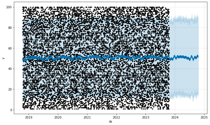
fig = model.plot_components(forecast)
plt.show()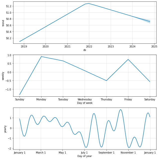
trend로 장기적인 경향을 시각화
Weekly Seasonality (주간 계절성) 요일별 주기적인 패턴 확인
Yearly Seasonality (연간 계절성) 월 또는 계절 단위의 반복되는 패턴을 시각화