import numpy as np
import matplotlib.pyplot as plt
from mpl_toolkits.mplot3d import Axes3DImport
Lecture 1
The fundamental Problem of Linear Algebra
n equations and n unknowns 특징 세 가지
1 행의 관점에서 바라보자
2 열의 관점에서 바라보자
3 A라고 부를거야
example 2 equations and 2 unknowns 이 있다면?
2 equations
\(2x - y = 0\)
\(-x + 2y =3\)
2 unknowns
\(x,y\)
\(\begin{bmatrix} 2 & -1 \\ -1 & 2 \end{bmatrix} \begin{bmatrix} x \\ y \end{bmatrix} = \begin{bmatrix} 0 \\ 3 \end{bmatrix}\) 로 나타낼 수 있고,
이는 이 식이 된다. \(A \bf{X}\) \(= b\)
- Row Picture
# 방정식의 계수 설정
A = np.array([[2, -1], [-1, 2]])
b = np.array([0, 3])

# 해 구하기
solution = np.linalg.solve(A, b)
x = np.linspace(-5, 5, 400)

# 그래프 그리기
plt.plot(x, 2*x, label='2x - y = 0')  # 첫 번째 방정식
plt.plot(x, (3 + x) / 2, label='-x + 2y = 3')  # 두 번째 방정식

# 해 표시
plt.plot(solution[0], solution[1], 'ro')  # 해는 빨간색으로 표시

# x=0, y=0에만 라인 추가
plt.axhline(0, color='black', linewidth=0.5)  # y=0
plt.axvline(0, color='black', linewidth=0.5)  # x=0

plt.xlabel('x')
plt.ylabel('y')
plt.grid(True)
plt.title('Row Picture of the Equations')
plt.legend()
plt.show()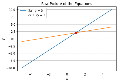
여기서 두 equation이 만나는 점인 \(\{ x=1, y=2 \}\)가 선형 결합(linear combination)이다.(이 점 외에는 만나지 않음!)
- Column Picture
\(x\begin{bmatrix} 2 \\ -1 \end{bmatrix} + y \begin{bmatrix} -1 \\ 2 \end{bmatrix} = \begin{bmatrix} 0 \\ 3 \end{bmatrix}\)
It is linear combination of columns.
우리는 이미 Row Picture에서 선형 결합 결과가 \(\{ x=1, y=2 \}\)라는 것을 아니까 대입해보면,
# 해벡터 계산
A = np.array([[2, -1], [-1, 2]])
b = np.array([0, 3])
solution = np.linalg.solve(A, b)
x = solution[0]
y = solution[1]

# col picture 그리기
plt.quiver(0, 0, A[0][0], A[1][0], angles='xy', scale_units='xy', scale=1, color='m', label='col1')
plt.quiver(0, 0, A[0][1], A[1][1], angles='xy', scale_units='xy', scale=1, color='c', label='col2')
plt.quiver(0, 0, x*A[0][0] + y*A[0][1], x*A[1][0] + y*A[1][1], angles='xy', scale_units='xy', scale=1, color='red', label='b = col1 + 2col2')
plt.quiver(x*A[0][0], x*A[1][0], y*A[0][1], y*A[1][1], angles='xy', scale_units='xy', scale=1, color='b', label='route')
plt.xlim(-5, 5)
plt.ylim(-5, 5)
plt.xlabel('x')
plt.ylabel('y')
plt.axhline(0, color='black',linewidth=0.5)
plt.axvline(0, color='black',linewidth=0.5)
plt.grid(color = 'gray', linestyle = '--', linewidth = 0.5)
plt.legend()
plt.title('Column Picture of the Equations')
plt.show()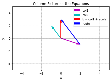
\(b\)인 \(x = 0, y = 3\)을 얻었다.
example 3 equations and 3 unknowns 이 있다면?
3 equations
\(2x - y = 0\)
\(-x + 2y - z = -1\)
\(-3y + 4z = 4\)
3 unknowns
\(x,y,z\)
\(A = \begin{bmatrix} 2 & -1 & 0 \\ -1 & 2 & -1 \\ 0 & -3 & 4 \end{bmatrix}, \bf{X}\) \(\begin{bmatrix}x \\ y \\ z \end{bmatrix}, b = \begin{bmatrix} 0 \\ -1 \\ 4 \end{bmatrix}\)
- Row Picture
3개의 different plane이 생성된다.
# 행렬과 벡터 정의
A = np.array([[2, -1, 0], [-1, 2, -1], [0, -3, 4]])
b = np.array([0, -1, 4])

# 해벡터 계산
solution = np.linalg.solve(A, b)

# 방정식을 풀어서 세 개의 평면을 정의
x = np.linspace(-10, 10, 10)
y = np.linspace(-10, 10, 10)
X, Y = np.meshgrid(x, y)

# 방정식들을 표현
Z1 = (2*X - Y) / 1
Z2 = (-X + 2*Y + 1) / 1
Z3 = (4/3)*Y + (4/3)

# Plotting row picture
fig = plt.figure(figsize=(10, 8))
ax = fig.add_subplot(111, projection='3d')

# Plotting planes
ax.plot_surface(X, Y, Z1, alpha=0.5)
ax.plot_surface(X, Y, Z2, alpha=0.5)
ax.plot_surface(X, Y, Z3, alpha=0.5)

# Plotting solution vector
ax.scatter(solution[0], solution[1], solution[2], color='r', s=100, label='Combination')

# Labels and legends
ax.set_xlabel('X-axis')
ax.set_ylabel('Y-axis')
ax.set_zlabel('Z-axis')
ax.set_title('Row Picture')
ax.legend()

plt.show()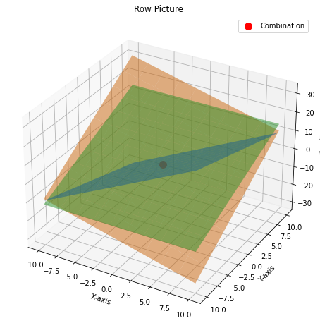
- Column Picture
각각 3 dimensional vector.
\(x\begin{bmatrix} 2 \\ -1 \\ 0 \end{bmatrix} + y \begin{bmatrix} -1 \\ 2 \\ -3 \end{bmatrix} + z \begin{bmatrix} 0 \\ -1 \\ 4 \end{bmatrix} = \begin{bmatrix} 0 \\ -1 \\ 4 \end{bmatrix}\)
- \(x=0,y=0,z=1\) 하면 b가 나오지 않아? 왜냐하면 col3은 b와 같으니까.
- \(b\)가 \(\begin{bmatrix} 1 \\ 1 \\ -3 \end{bmatrix}\) 이라면? \(x=1,y=1,z=0\) 이겠지?
# 주어진 벡터와 결과 벡터 정의
v1 = np.array([2, -1, 0])
v2 = np.array([-1, 2, -3])
v3 = np.array([0, -1, 4])
result_vector = np.array([0, -1, 4])

# 그래프 생성
fig = plt.figure(figsize=(10, 8))
ax = fig.add_subplot(111, projection='3d')

# 벡터 그리기
ax.quiver(0, 0, 0, v1[0], v1[1], v1[2], color='r', label='v1', arrow_length_ratio=0.1)
ax.quiver(0, 0, 0, v2[0], v2[1], v2[2], color='g', label='v2', arrow_length_ratio=0.1)
ax.quiver(0, 0, 0, v3[0], v3[1], v3[2], color='b', label='v3', arrow_length_ratio=0.1)

# 결과 벡터 그리기
ax.quiver(0, 0, 0, result_vector[0], result_vector[1], result_vector[2], color='k', label='Result', arrow_length_ratio=0.1)

# 축 범위 설정
ax.set_xlim([-1, 2])
ax.set_ylim([-1, 3])
ax.set_zlim([-4, 2])

# 축 레이블
ax.set_xlabel('X-axis')
ax.set_ylabel('Y-axis')
ax.set_zlabel('Z-axis')

# 그래프 표시
ax.legend()
plt.title('Column Picture')
plt.show()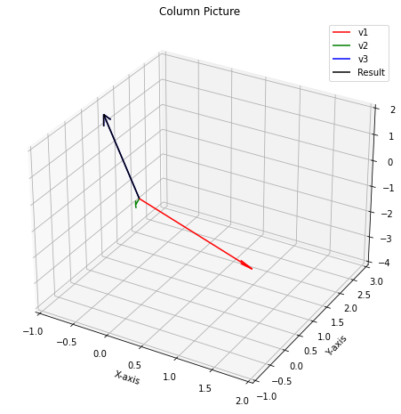
-
- Can I solve \(A\bf{X}\) \(=b\) for every \(b\)?
- 아닌듯, 예, unknowns가 서로 연관있다면?
- 만약 이 3 equations 3 unknows에서 이 세 columns가 same plane에 놓여있다면, 그들의 combination도 same plane에 놓일 것이다. -> 문제 발생!
- col1 = col2 = col3 이렇게 같은 plane이면 새로운 값 b를 얻지 못한다.
대부분의 right hand side는 out pf plane 이거나 unreachable 하다. -> singular case , not invertible
- There would not be a solution for every b
example 9 dimensions 라면?
- 9 vectors, 9 dimensional space 나오겠지.
Can we get every right hand side?
depending on those nine columns
columns가 independent 하지 않다면 new b를 얻지 못해서 b를 못 구한다.
- check
dimension이 점점 커지면 row picture는 어떻게 표현할 것인가?
column picture 는 벡터로 표현하는 것이기 때문에 어려움 없이 선형 결합 linear combination 표현 가능.
\(AX\) is a combination of columns of \(A\)