GODE에서 사용된 Graph signal 예제들에 대한 설명

Import

import pickle

Esmaple 1. Simple Linear

Data Information

\(V=\{{\boldsymbol v}_1,\dots,{\boldsymbol v}_n\}:=\{(x_1,y_2,z_3),\dots,(x_n,y_n,z_n)\}\)
- \(r_i= 5 + \cos(\frac{12\pi (i - 1)}{n - 1})\), \(\theta_i= -\pi + \frac{{\pi(n-2)(i - 1)}}{n(n - 1)}\)
- \(x_i = r_i \cos(\theta_i)\), \(y_i = r_i \sin(\theta_i)\), \(z_i = 10 \cdot \sin(\frac{{6\pi \cdot (i - 1)}}{{n - 1}})\).
\(W_{i,j} = \begin{cases} \exp\left(-\frac{\|{\boldsymbol v}_i -{\boldsymbol v}_j\|^2}{2\theta^2}\right) & \|{\boldsymbol v}_i -{\boldsymbol v}_j\|^2 \le \kappa \\ 0 & o.w\end{cases}\)

Note that \({\bf L}\) is GSO, and in this case, GFT is just Discrete Fourier Transform also note that \({\cal G}_W\) is a regular graph since \({\bf D}={\bf I}\). Thus this data is Euclidean data.

graph signal

\(y:V \to \mathbb{R}\)

\(y_i=\frac{10}{n}v_i+\eta_i+\epsilon_i\)
\(\epsilon_i \sim N(\mu,\sigma^2)\)
\(\eta_i \sim U^\star\) with sparsity \(0.05\) where \(U^\star\) is mixture of \(U(1.5,2)\) and \(U(-2,-1.5)\).

Note that \({\bf y}\) is weakly stationary w.r.t. \({\bf L}\).

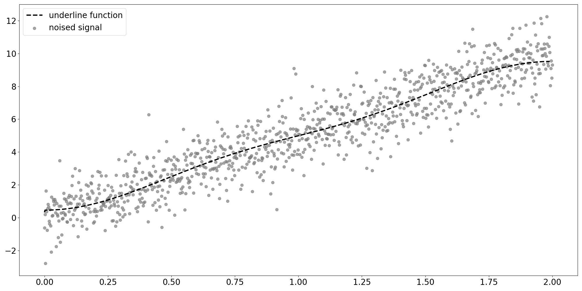
Euclidean Data

domain 이 \(x\)축(실수 \(\mathbb{R}\)로 정의되는)인 유클리디안 데이터
underline이 선, 아래에서는 \(y=5x\)가 되겠다.
- 1d-grid로 볼 수 있음.(non-euclidean vs euclidean 참고)
underliying function이 regular graph로 정의(regular graph 참고)

Esmaple 2. Orbit

Data Information

\({\cal G}_W=(V,E,{\bf W})\)

\(V=\{{\boldsymbol v}_1,\dots,{\boldsymbol v}_n\}:=\{(x_1,y_2,z_3),\dots,(x_n,y_n,z_n)\}\)
- \(r_i= 5 + \cos(\frac{12\pi (i - 1)}{n - 1})\), \(\theta_i= -\pi + \frac{{\pi(n-2)(i - 1)}}{n(n - 1)}\)
- \(x_i = r_i \cos(\theta_i)\), \(y_i = r_i \sin(\theta_i)\), \(z_i = 10 \cdot \sin(\frac{{6\pi \cdot (i - 1)}}{{n - 1}})\).
\(W_{i,j} = \begin{cases} \exp\left(-\frac{\|{\boldsymbol v}_i -{\boldsymbol v}_j\|^2}{2\theta^2}\right) & \|{\boldsymbol v}_i -{\boldsymbol v}_j\|^2 \le \kappa \\ 0 & o.w\end{cases}\)

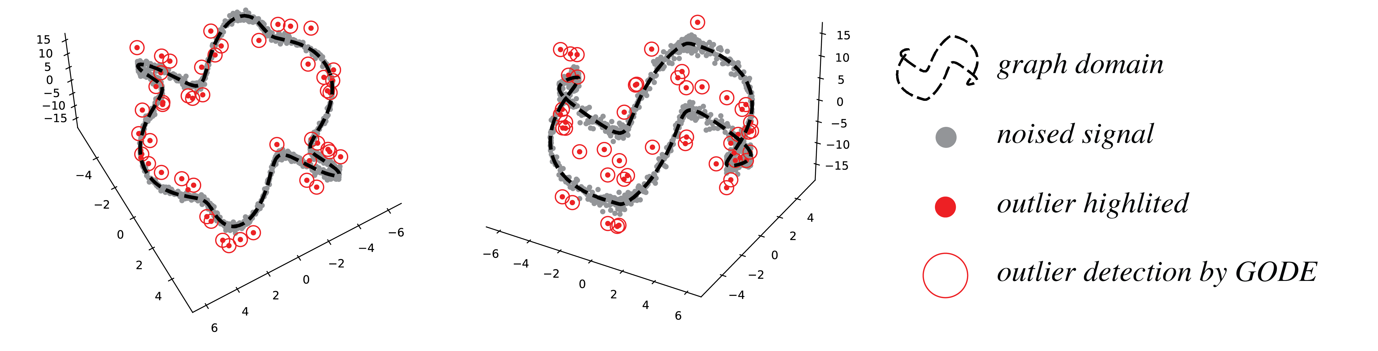
Non-Euclidean Data

2D shape이다.
domain이 곡선인 논유클리디안 데이터
underlying function이 regular graph로 정의되지 않는다.(regular graph 참고)
거리 계산을 유클리드 거리로 할 때, underline이 곡선이라 합리적이지 않다.
weight은 유클리디안 거리로 정의되어 있지만, \(\kappa\)로 hyperparameter 지정해주어 거리가 짧으면 유클리디안 거리로 정의하고, 멀면 0으로 연결을 끊는 행렬으로 정의.

Note

유클리디안으로 보고 싶다면??

모든 연결 weight를 끊어버리면 된다.
그러면 regular graph 로 정의 가능.
하지만, d연구의 목적에 어긋남.

Note that \({\bf W}\) is GSO, since \({\bf W}^\top = {\bf W}\). In this cases, \({\cal G}_W\) is not regular since there does not exist \(k\) such that \({\bf D}=k{\bf I}\).

graph signal \({\bf y}:V \to \mathbb{R}^3\)

\({\bf y}_i={\boldsymbol v}_i+{\boldsymbol \eta}_i+{\boldsymbol \epsilon}_i\)
\({\boldsymbol \epsilon}_i \sim N({\boldsymbol \mu},\sigma^2{\bf I})\)
\({\boldsymbol \eta}_i \sim U^\star\) with sparsity \(0.05\) where \(U^\star\) is mixture of \(U(5,7)\) and \(U(-7,-5)\).

Clearly \({\bf y}\) is stationary w.r.t. \({\bf W}\) or \({\bf L}\).

Esmaple 3. Stanford Bunny

Data Information

pygsp 라이브러리를 사용하여 데이터 가져옴, weight도!(mesh 로 색의 퍼짐 정도로 나타낸 것으로 간단 이해)

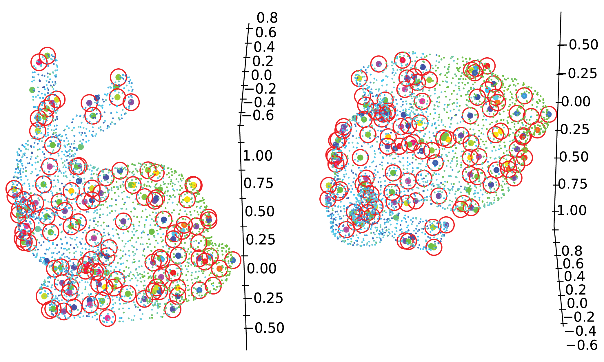
Non-Euclidean Data

3D shape
domain이 곡면이고, underline이 곡면인 넌유클리디안 데이터
underlying function 이 색
- 아래를 설명해보자면, 연한 파란-연한 초록 점이 언더라인 펑션으로 형성되어 있을때, 진한 색의 점들이 noise로 형성되어 있음.
underline이 곡면이라 유클리디안 거리를 사용하는 것이 합리적이지 않다.

Real data. Earthquake

Data Information

This data is actual data collected from USGS¹ during the period from 2010 to 2014.

\({\cal G}=(V,E)\)

\(V=\{{\boldsymbol v}_1,\dots,{\boldsymbol v}_n\}\) where \({\boldsymbol v}:=({\tt Latitude},{\tt Longitude})\)
\(W_{i,j} = \begin{cases} \exp(-\frac{\rho(i,j)}{2\theta^2}) & if \rho(i,j) \le \kappa \\ 0 & o.w. \end{cases}\)
- Here, \(\rho(i,j)=hs({\boldsymbol v}_i, {\boldsymbol v}_j)\) is Haversine distance between \({\boldsymbol v}_i, {\boldsymbol v}_j\).
\(y_i\) = magnitude

Non-Euclidean Data

domain이 곡면이고, underline이 곡면인 넌유클리디안 데이터
underlying function 이 magnitude(지진 강도)
haversine 이용하면 곡면 거리가 이미 포함되어 있지만, 자료가 너무 많아 거리가 먼 연결을 끊어주는 역할로 hyperparameter인 \(\kappa\)사용하였다.

with open("Figs/GODE_earthquake.pkl", "rb") as file:
    loaded_object = pickle.load(file)

loaded_object

Footnotes

https://www.usgs.gov/programs/earthquake-hazards/lists-maps-and-statistics↩︎