import GODEThis tutorial is about GODE: Graph fourier transform based Outlier Detection using Emprical Bayesian thresholding paper.
0. Import
Import the necessary packages.
import numpy as np
import pandas as pd
from pygsp import graphs, filters, plotting, utils1. Linear
1.1. Data
Data description
- Graph \({\cal G}_W=(V,E,{\bf W})\)
- Vertex set \(V=\{1,2,\dots,n\}\)
- \(n=1000\)
- \(W_{ij} = \begin{cases} 1, & \text{ if } j-i = 1 \\ 0, & \text{ otherwise}\end{cases}\)
- Graph signal \(y:V \to \mathbb{R}\)
\[y_i=\frac{10}{n}v_i+\eta_i+\epsilon_i,\]
- \(v_i = v_1, v_2, \ldots, v_n\)
- \(\eta_i = \begin{cases} U(5,7) & \text{ with probability 0.025}\\ U(-7,-5) & \text{ with probability 0.025} \\ 0 & \text{ otherwise } \end{cases}\)
- \(\epsilon_i \sim N(\mu,\sigma^2)\)
np.random.seed(6)
epsilon = np.around(np.random.normal(size=1000),15)
signal = np.random.choice(np.concatenate((np.random.uniform(-7, -5, 25).round(15), np.random.uniform(5, 7, 25).round(15), np.repeat(0, 950))), 1000)
eta = signal + epsilon

outlier_true_linear= signal.copy()
outlier_true_linear = list(map(lambda x: 1 if x!=0 else 0,outlier_true_linear))
index_of_trueoutlier_bool = signal!=0
x_1 = np.linspace(0,2,1000)
y1_1 = 5 * x_1
y_1 = y1_1 + eta # eta = signal + epsilon
_df=pd.DataFrame({'x':x_1, 'y':y_1})1.2. GODE
Lin = GODE.Linear(_df)Lin.fit(sd=20)outlier_old_linear, outlier_linear, outlier_index_linear = GODE.GODE_Anomalous(Lin(_df),contamination=0.05)1.3. Plot
GODE.Linear_plot(Lin(_df),index_of_trueoutlier_bool, outlier_index_linear)
Lin(_df)['x'][:10]array([0. , 0.002002 , 0.004004 , 0.00600601, 0.00800801,
0.01001001, 0.01201201, 0.01401401, 0.01601602, 0.01801802])Lin(_df)['y'][:10]array([-0.31178367, -6.08358567, 0.23784081, -0.86906177, -2.44674061,
0.96330157, 1.18712379, -1.44402316, 1.71937116, -0.33980351])Lin(_df)['yhat'][:10]array([0.26224717, 0.37091714, 0.37104804, 0.3712662 , 0.3715716 ,
0.37196424, 0.37244408, 0.37301111, 0.3736653 , 0.37440661])1.4. Confusion matrix
Conf_linear = GODE.Conf_matrx(outlier_true_linear,outlier_linear)Conf_linear.conf('GODE')
Accuracy: 0.999
Precision: 1.000
Recall: 0.980
F1 Score: 0.990Conf_linear(){'Accuracy': 0.999,
'Precision': 1.0,
'Recall': 0.9803921568627451,
'F1 Score': 0.99009900990099}2. Orbit
2.1. Data
Data description
- Graph \({\cal G}_W=(V,E,{\bf W})\)
- Vertex set \(V=\{1,2,\dots,n\}\)
- \({\bf W} = \begin{cases} \exp\left(-\frac{|{\boldsymbol v}_i -{\boldsymbol v}_j|^2}{2\theta^2}\right), & \text{ if } |{\boldsymbol v}_i - {\boldsymbol v}_j| \le \kappa \\ 0, & \text{ otherwise}\end{cases}\)
- \(\theta=6.45\) and \(\kappa=2500\)
- \(n=1000\)
- graph signal \(y:V \to \mathbb{R}\)
\[y_i = 10 \cdot \sin\left(\frac{{6\pi \cdot (i - 1)}}{{n - 1}}\right)+\epsilon_i+\eta_i\]
- \({\boldsymbol v}_i=(x_i,y_i)\)
- \(x_i = r_i \cos(\theta_i)\)
- \(y_i = r_i \sin(\theta_i)\)
- \(r_i= 5 + \cos(\frac{12\pi (i - 1)}{n - 1})\)
- \(\theta_i= -\pi + \frac{{\pi(n-2)(i - 1)}}{n(n - 1)}\)
- \(\eta_i = \begin{cases} U(1,4) & \text{ with probability 0.025}\\ U(-4,-1) & \text{ with probability 0.025} \\ 0 & \text{ otherwise } \end{cases}\)
- \(\epsilon_i \sim N(\mu,\sigma^2)\)
np.random.seed(777)
epsilon = np.around(np.random.normal(size=1000),15)
signal = np.random.choice(np.concatenate((np.random.uniform(-4, -1, 25).round(15), np.random.uniform(1, 4, 25).round(15), np.repeat(0, 950))), 1000)
eta = signal + epsilon
pi=np.pi
n=1000
ang=np.linspace(-pi,pi-2*pi/n,n)
r=5+np.cos(np.linspace(0,12*pi,n))
vx=r*np.cos(ang)
vy=r*np.sin(ang)
f1=10*np.sin(np.linspace(0,6*pi,n))
f = f1 + eta
_df = pd.DataFrame({'x' : vx, 'y' : vy, 'f1':f1, 'f' : f})
outlier_true_orbit = signal.copy()
outlier_true_orbit = list(map(lambda x: 1 if x!=0 else 0,outlier_true_orbit))
index_of_trueoutlier_bool = signal!=0
2.2. GODE
Or = GODE.Orbit(_df)Or.fit(sd=15,method = 'Euclidean')100%|██████████| 1000/1000 [00:01<00:00, 613.53it/s]outlier_old_orbit, outlier_orbit, outlier_index_orbit = GODE.GODE_Anomalous(Or(_df),contamination=0.05)2.3. Plot
GODE.Orbit_plot(Or(_df),index_of_trueoutlier_bool,outlier_index_orbit)
Or(_df)['x'][:5]array([-6. , -5.99916963, -5.9966797 , -5.99253378, -5.98673778])Or(_df)['y'][:5]array([-7.34788079e-16, -3.76943905e-02, -7.53604665e-02, -1.12969981e-01,
-1.50494820e-01])Or(_df)['f1'][:5]array([0. , 0.18867305, 0.37727893, 0.56575049, 0.75402065])Or(_df)['f'][:5]array([-0.46820879, -0.63415181, 0.31189882, -0.14761143, 1.66037153])Or(_df)['fhat'][:5]array([0.08086037, 0.2425556 , 0.40437747, 0.5665164 , 0.72915801])2.4. Confusion matrix
Conf_orbit = GODE.Conf_matrx(outlier_true_orbit,outlier_orbit)Conf_orbit.conf('GODE')
Accuracy: 0.955
Precision: 0.540
Recall: 0.551
F1 Score: 0.545Conf_orbit(){'Accuracy': 0.955,
'Precision': 0.54,
'Recall': 0.5510204081632653,
'F1 Score': 0.5454545454545455}3. Bunny
3.1. Data
Data description
- Stanford bunny data
- \(n=2503\)
G = graphs.Bunny()
n = G.N
g = filters.Heat(G, tau=75)
n=2503
np.random.seed(1212)
normal = np.around(np.random.normal(size=n),15)
unif = np.concatenate([np.random.uniform(low=3,high=7,size=60), np.random.uniform(low=-7,high=-3,size=60),np.zeros(n-120)]); np.random.shuffle(unif)
noise = normal + unif
f = np.zeros(n)
f[1000] = -3234
f = g.filter(f, method='chebyshev')
outlier_true_bunny = unif.copy()
outlier_true_bunny = list(map(lambda x: 1 if x !=0  else 0,outlier_true_bunny))
index_of_trueoutlier_bool_bunny = unif!=0
2023-11-30 13:14:41,369:[WARNING](pygsp.graphs.graph.lmax): The largest eigenvalue G.lmax is not available, we need to estimate it. Explicitly call G.estimate_lmax() or G.compute_fourier_basis() once beforehand to suppress the warning.G.coords.shape
_W = G.W.toarray()
_x = G.coords[:,0]
_y = G.coords[:,1]
_z = -G.coords[:,2]
_df = pd.DataFrame({'x':_x,'y':_y,'z':_z, 'f1' : f, 'f':f+noise,'noise': noise})3.2. GODE
bu = GODE.BUNNY(_df,_W)bu.fit(sd=20)outlier_old_bunny, outlier_bunny, outlier_index_bunny = GODE.GODE_Anomalous(bu(_df),contamination=0.05)3.3. Plot
GODE.Bunny_plot(bu(_df),index_of_trueoutlier_bool_bunny,outlier_index_bunny)
bu(_df){'x': array([ 0.26815193, -0.58456893, -0.02730755, ..., 0.15397547,
-0.45056488, -0.29405249]),
'y': array([ 0.39314334, 0.63468595, 0.33280949, ..., 0.80205526,
0.6207154 , -0.40187451]),
'z': array([-0.13834514, -0.22438843, 0.08658215, ..., 0.33698514,
0.58353051, -0.08647485]),
'f1': array([-1.54422488, -0.03596483, -0.93972715, ..., -0.01924028,
-0.02470869, -0.26266752]),
'f': array([-0.8068728 , -0.65326195, -4.41287087, ..., -2.06257107,
0.72882576, -0.47420275]),
'fhat': array([-1.82796431, 0.04748775, -1.12152947, ..., -0.03652692,
0.06627654, 0.1743586 ])}3.4. Confusion matrix
Conf_bunny = GODE.Conf_matrx(outlier_true_bunny,outlier_bunny)Conf_bunny.conf('GODE')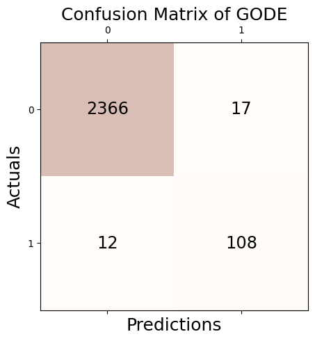
Accuracy: 0.988
Precision: 0.864
Recall: 0.900
F1 Score: 0.882Conf_bunny(){'Accuracy': 0.9884139033160207,
'Precision': 0.864,
'Recall': 0.9,
'F1 Score': 0.8816326530612244}4. Earthquake
4.1. Data
Data description
USGS data from \(2010\) to \(2014\)
Graph \({\cal G}=(V,E,{\bf W})\)
Vertex set \(V = \{v_1, v_2, \ldots, v_n\}\)
\(v:= \tt{( Latitude}\), \(\tt{Longitude)}\)
\(n=10762\)
\({\bf W_{ij}} = \begin{cases} \exp(-\frac{\rho(i,j)}{2 \theta^2}), & \text{ if } |\rho(i,j)| \le \kappa \\ 0, & \text{ otherwise}\end{cases}\)
\(\rho(i,j)=hs({\boldsymbol v}_i, {\boldsymbol v}_j)\)
\(\theta = 8810.87\) and \(\kappa = 2500\)
graph signal \(y:V \to \mathbb{R}\)
_df = pd.read_csv('./earthquake_tutorial.csv')_df = _df.assign(Year=list(map(lambda x: x.split('-')[0], _df.time))).rename(columns={'latitude' : 'x', 'longitude' : 'y', 'mag': 'f'}).iloc[:,1:]
_df.Year = _df.Year.astype(np.float64)4.2. GODE
Er = GODE.Earthquake(_df.query("2010 <= Year < 2011"))Er.fit(sd=20, method = 'Haversine')100%|██████████| 4790/4790 [00:30<00:00, 158.67it/s]Er(_df.query("2010 <= Year < 2011")){'x': array([ 0.663, -19.209, -31.83 , ..., 40.726, 30.646, 26.29 ]),
'y': array([ -26.045, 167.902, -178.135, ..., 51.925, 83.791, 99.866]),
'f': array([5.5, 5.1, 5. , ..., 5. , 5.2, 5. ]),
'fhat': array([5.62793904, 5.15719404, 4.99555904, ..., 5.42038559, 5.27983909,
5.08949907])}outlier_old_earthquake, outlier_earthquake, outlier_index_earthquake = GODE.GODE_Anomalous(Er(_df.query("2010 <= Year < 2011")),contamination=0.05)4.3. Plot
GODE.Earthquake_plot(Er(_df.query("2010 <= Year < 2011")),outlier_index_earthquake,lat_center=37.7749, lon_center=-122.4194,fThresh=7,adjzoom=5,adjmarkersize = 40)