import networkx as nx
import matplotlib.pyplot as plt
import numpy as np
from tqdm import tqdm
from torch_geometric_temporal.signal import temporal_signal_splitPyTorch ST-GCN Dataset
ST-GCN
PyTorch Geometric Temporal Dataset
https://pytorch-geometric-temporal.readthedocs.io/en/latest/modules/dataset.html#module-torch_geometric_temporal.dataset.chickenpox
|Dataset|Signal|Graph|Frequency|𝑇|ㅣ𝑉ㅣ | |:–:|:–:||:–:||:–:| |Chickenpox Hungary|Temporal|Static|Weekly|522|20| |Windmill Large|Temporal|Static|Hourly|17,472|319| |Windmill Medium|Temporal|Static|Hourly|17,472|26| |Windmill Small|Temporal|Static|Hourly|17,472|11| |Pedal Me Deliveries|Temporal|Static|Weekly|36|15| |Wikipedia Math|Temporal|Static|Daily|731|1,068| |Twitter Tennis RG|Static|Dynamic|Hourly|120|1000| |Twitter Tennis UO|Static|Dynamic|Hourly|112|1000| |Covid19 England|Temporal|Dynamic|Daily|61|129| |Montevideo Buses|Temporal|Static|Hourly|744|675| |MTM-1 Hand Motions|Temporal|Static|1/24 Seconds|14,469|21|
RecurrentGCN
import torch
import torch.nn.functional as F
from torch_geometric_temporal.nn.recurrent import GConvGRU

class RecurrentGCN(torch.nn.Module):
    def __init__(self, node_features, filters):
        super(RecurrentGCN, self).__init__()
        self.recurrent = GConvGRU(node_features, filters, 2)
        self.linear = torch.nn.Linear(filters, 1)

    def forward(self, x, edge_index, edge_weight):
        h = self.recurrent(x, edge_index, edge_weight)
        h = F.relu(h)
        h = self.linear(h)
        return h
ChickenpoxDatasetLoader
Chickenpox Hungary
- A spatiotemporal dataset about the officially reported cases of chickenpox in Hungary. The nodes are counties and edges describe direct neighbourhood relationships. The dataset covers the weeks between 2005 and 2015 without missingness.
데이터정리
- T = 519
- N = 20 # number of nodes
- E = 102 # edges
- \(f(v,t)\)의 차원? (1,)
- 시간에 따라서 Number of nodes가 변하는지? False
- 시간에 따라서 Number of nodes가 변하는지? False
- X: (20,4) (N,4), \(f(v,t_0),f(v,t_1),f(v,t_2),f(v,t_3)\)
- y: (20,) (N,), \(f(v,t_4)\)
- 예제코드적용가능여부: Yes
- Nodes : 20
- vertices are counties
-Edges : 102
- edges are neighbourhoods
- Time : 519
- between 2004 and 2014
- per weeks
from torch_geometric_temporal.dataset import  ChickenpoxDatasetLoader
from torch_geometric_temporal.signal import temporal_signal_split

loader = ChickenpoxDatasetLoader()

dataset = loader.get_dataset(lags=1)

train_dataset, test_dataset = temporal_signal_split(dataset, train_ratio=1)data=[]
for time, snapshot in enumerate(train_dataset):
data.append([time,snapshot])time519(data[0][1]).x.type,(data[0][1]).edge_index.type,(data[0][1]).edge_attr.type,(data[0][1]).y.type(<function Tensor.type>,
<function Tensor.type>,
<function Tensor.type>,
<function Tensor.type>)max((data[4][1]).x[0])tensor(2.1339)G = nx.Graph()node_list = torch.tensor(range(20)).tolist()G.add_nodes_from(node_list)data[-1][519, Data(x=[20, 1], edge_index=[2, 102], edge_attr=[102], y=[20])]len(data[0][1].edge_index[0])102edge_list=[]
for i in range(519):
for j in range(len(data[0][1].edge_index[0])):
edge_list.append([data[i][1].edge_index[0][j].tolist(),data[i][1].edge_index[1][j].tolist()])G.add_edges_from(edge_list)G.number_of_nodes(),G.number_of_edges()(20, 61)nx.draw(G,with_labels=True,font_weight='bold',node_color='green',node_size=350,font_color='white',width=1)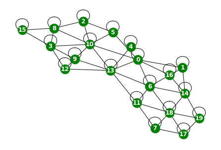
time별 같은 edge 정보를 가지고 있나 확인
np.where(data[0][1].edge_index != data[10][1].edge_index)(array([], dtype=int64), array([], dtype=int64))from torch_geometric_temporal.dataset import ChickenpoxDatasetLoader
loader = ChickenpoxDatasetLoader()
dataset = loader.get_dataset(lags=4)
train_dataset, test_dataset = temporal_signal_split(dataset, train_ratio=0.5)data=[]
for time, snapshot in enumerate(train_dataset):
data.append([time,snapshot])(data[0][1]).x[0], (data[0][1]).y[0](tensor([-0.0011, 0.0286, 0.3547, 0.2954]), tensor(0.7106))\(t=0\)에서 \(X\)와 \(y\)를 정리하면 아래와 같음.
- X:= \(x_0,x_1,x_2,x_3\)
- y:= \(x_4\)
(data[1][1]).x[0]tensor([0.0286, 0.3547, 0.2954, 0.7106])- X:= \(x_1,x_2,x_3,x_4\)
- y:= \(x_5\)
(data[2][1]).x[0]tensor([ 0.3547, 0.2954, 0.7106, -0.6831])- X:=\(x_2,x_3,x_4,x_5\)
- y:=\(x_6\)
하나의 노드에 길이가 \(T\)인 시계열이 맵핑되어 있음. (노드는 총 20개)
각 노드마다 아래와 같은 과정으로 예측이 됨
- \((x_0,x_1,x_2,x_3) \to (x_4)\)
- \((x_1,x_2,x_3,x_4) \to (x_5)\)
\(f(v,t), v \in \{v_1,\dots,v_{20}\}, t=1,2,\dots,519\)
\[{\bf X}_{t=1} = \begin{bmatrix} f(v_1,t=1) & f(v_1,t=2) & f(v_1,t=3)& f(v_1,t=4) \\ f(v_2,t=1) & f(v_2,t=2) & f(v_2,t=3)& f(v_2,t=4) \\ \dots & \dots & \dots & \dots \\ f(v_{20},t=1) & f(v_{20},t=2) & f(v_{20},t=3)& f(v_{20},t=4) \end{bmatrix}\]
\[{\bf y}_{t=1} = \begin{bmatrix} f(v_1,t=5) \\ f(v_2,t=5) \\ \dots \\ f(v_{20},t=5) \end{bmatrix}\]
Learn
model = RecurrentGCN(node_features=4, filters=32)
optimizer = torch.optim.Adam(model.parameters(), lr=0.01)
model.train()
for epoch in tqdm(range(50)):
for time, snapshot in enumerate(train_dataset):
y_hat = model(snapshot.x, snapshot.edge_index, snapshot.edge_attr)
cost = torch.mean((y_hat-snapshot.y)**2)
cost.backward()
optimizer.step()
optimizer.zero_grad()100%|██████████| 50/50 [00:52<00:00, 1.05s/it]for time, snapshot in enumerate(train_dataset):
_x = snapshot.x
_edge_index = snapshot.edge_index
_edge_attr = snapshot.edge_attr
_y = snapshot.y
break_x.shapetorch.Size([20, 4])_edge_index.shapetorch.Size([2, 102])_edge_attr.shapetorch.Size([102])_y.shapetorch.Size([20])_x.shapetorch.Size([20, 4])x
Vertex features are lagged weekly counts of the chickenpox cases (we included 4 lags). y
The target is the weekly number of cases for the upcoming week
_xtensor([[-1.0814e-03, 2.8571e-02, 3.5474e-01, 2.9544e-01],
[-7.1114e-01, -5.9843e-01, 1.9051e-01, 1.0922e+00],
[-3.2281e+00, -2.2910e-01, 1.6103e+00, -1.5487e+00],
[ 6.4750e-01, -2.2117e+00, -9.6858e-01, 1.1862e+00],
[-1.7302e-01, -9.4717e-01, 1.0347e+00, -6.3751e-01],
[ 3.6345e-01, -7.5468e-01, 2.9768e-01, -1.6273e-01],
[-3.4174e+00, 1.7031e+00, -1.6434e+00, 1.7434e+00],
[-1.9641e+00, 5.5208e-01, 1.1811e+00, 6.7002e-01],
[-2.2133e+00, 3.0492e+00, -2.3839e+00, 1.8545e+00],
[-3.3141e-01, 9.5218e-01, -3.7281e-01, -8.2971e-02],
[-1.8380e+00, -5.8728e-01, -3.5514e-02, -7.2298e-02],
[-3.4669e-01, -1.9827e-01, 3.9540e-01, -2.4774e-01],
[ 1.4219e+00, -1.3266e+00, 5.2338e-01, -1.6374e-01],
[-7.7044e-01, 3.2872e-01, -1.0400e+00, 3.4945e-01],
[-7.8061e-01, -6.5022e-01, 1.4361e+00, -1.2864e-01],
[-1.0993e+00, 1.2732e-01, 5.3621e-01, 1.9023e-01],
[ 2.4583e+00, -1.7811e+00, 5.0732e-02, -9.4371e-01],
[ 1.0945e+00, -1.5922e+00, 1.3818e-01, 1.1855e+00],
[-7.0875e-01, -2.2460e-01, -7.0875e-01, 1.5630e+00],
[-1.8228e+00, 7.8633e-01, -5.6172e-01, 1.2647e+00]])_ytensor([ 0.7106, -0.0725, 2.6099, 1.7870, 0.8024, -0.2614, -0.8370, 1.9674,
-0.4212, 0.1655, 1.2519, 2.3743, 0.7877, 0.4531, -0.1721, -0.0614,
1.0452, 0.3203, -1.3791, 0.0036])PedalMeDatasetLoader
Pedal Me Deliveries
- A dataset about the number of weekly bicycle package deliveries by Pedal Me in London during 2020 and 2021. Nodes in the graph represent geographical units and edges are proximity based mutual adjacency relationships.
데이터정리
- T = 33
- V = 지역의 집합
- N = 15 # number of nodes
- E = 225 # edges
- \(f(v,t)\)의 차원? (1,) # number of deliveries
- 시간에 따라서 N이 변하는지? False
- 시간에 따라서 E가 변하는지? False
- X: (15,4) (N,4), \(f(v,t_0),f(v,t_1),f(v,t_2),f(v,t_3)\)
- y: (15,) (N,), \(f(v,t_4)\)
- 예제코드적용가능여부: Yes
- Nodes : 15
- vertices are localities
-Edges : 225
- edges are spatial_connections
- Time : 33
- between 2020 and 2021
- per weeks
from torch_geometric_temporal.dataset import PedalMeDatasetLoader
from torch_geometric_temporal.signal import temporal_signal_split
loader = PedalMeDatasetLoader()
dataset = loader.get_dataset(lags=1)
train_dataset, test_dataset = temporal_signal_split(dataset, train_ratio=1)data=[]
for time, snapshot in enumerate(train_dataset):
data.append([time,snapshot])time33(data[0][1]).x.shape,(data[0][1]).edge_index.shape,(data[0][1]).edge_attr.shape(torch.Size([15, 1]), torch.Size([2, 225]), torch.Size([225]))G = nx.Graph()node_list = torch.tensor(range(15)).tolist()G.add_nodes_from(node_list)data[-1][33, Data(x=[15, 1], edge_index=[2, 225], edge_attr=[225], y=[15])]edge_list=[]
for i in range(33):
for j in range(len(data[0][1].edge_index[0])):
edge_list.append([data[i][1].edge_index[0][j].tolist(),data[i][1].edge_index[1][j].tolist()])G.add_edges_from(edge_list)G.number_of_nodes(),G.number_of_edges()(15, 120)nx.draw(G,with_labels=True,font_weight='bold',node_color='green',node_size=350,font_color='white',width=1)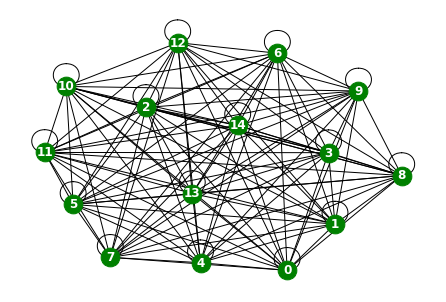
time별 같은 edge 정보를 가지고 있나 확인
np.where(data[0][1].edge_index != data[10][1].edge_index)(array([], dtype=int64), array([], dtype=int64))from torch_geometric_temporal.dataset import PedalMeDatasetLoader
loader = PedalMeDatasetLoader()
dataset = loader.get_dataset(lags=4)
train_dataset, test_dataset = temporal_signal_split(dataset, train_ratio=0.5)data=[]
for time, snapshot in enumerate(train_dataset):
data.append([time,snapshot])(data[0][1]).x[0], (data[0][1]).y[0](tensor([ 3.0574, -0.0477, -0.3076, 0.2437]), tensor(-0.2710))\(t=0\)에서 \(X\)와 \(y\)를 정리하면 아래와 같음.
- X:= \(x_0,x_1,x_2,x_3\)
- y:= \(x_4\)
(data[1][1]).x[0], (data[1][1]).y[0](tensor([-0.0477, -0.3076, 0.2437, -0.2710]), tensor(0.2490))- X:= \(x_1,x_2,x_3,x_4\)
- y:= \(x_5\)
(data[2][1]).x[0], (data[2][1]).y[0](tensor([-0.3076, 0.2437, -0.2710, 0.2490]), tensor(-0.0357))- X:=\(x_2,x_3,x_4,x_5\)
- y:=\(x_6\)
하나의 노드에 길이가 \(T\)인 시계열이 맵핑되어 있음. (노드는 총 15개)
각 노드마다 아래와 같은 과정으로 예측이 됨
- \((x_0,x_1,x_2,x_3) \to (x_4)\)
- \((x_1,x_2,x_3,x_4) \to (x_5)\)
\(f(v,t), v \in \{v_1,\dots,v_{15}\}, t=1,2,\dots,33\)
\[{\bf X}_{t=1} = \begin{bmatrix} f(v_1,t=1) & f(v_1,t=2) & f(v_1,t=3)& f(v_1,t=4) \\ f(v_2,t=1) & f(v_2,t=2) & f(v_2,t=3)& f(v_2,t=4) \\ \dots & \dots & \dots & \dots \\ f(v_{20},t=1) & f(v_{20},t=2) & f(v_{20},t=3)& f(v_{20},t=4) \end{bmatrix}\]
\[{\bf y}_{t=1} = \begin{bmatrix} f(v_1,t=5) \\ f(v_2,t=5) \\ \dots \\ f(v_{20},t=5) \end{bmatrix}\]
Learn
model = RecurrentGCN(node_features=4, filters=32)
optimizer = torch.optim.Adam(model.parameters(), lr=0.01)
model.train()
for epoch in tqdm(range(50)):
for time, snapshot in enumerate(train_dataset):
y_hat = model(snapshot.x, snapshot.edge_index, snapshot.edge_attr)
cost = torch.mean((y_hat-snapshot.y)**2)
cost.backward()
optimizer.step()
optimizer.zero_grad()100%|██████████| 50/50 [00:03<00:00, 16.04it/s]for time, snapshot in enumerate(train_dataset):
_x = snapshot.x
_edge_index = snapshot.edge_index
_edge_attr = snapshot.edge_attr
_y = snapshot.y
break_x.shapetorch.Size([15, 4])_edge_index.shapetorch.Size([2, 225])_edge_attr.shapetorch.Size([225])_y.shapetorch.Size([15])_x.shapetorch.Size([15, 4])x
- Vertex features are lagged weekly counts of the delivery demands (we included 4 lags).
- 주마다 배달 수요의 수가 얼마나 될지 percentage로, t-4시점까지?
y
- The target is the weekly number of deliveries the
upcomingweek. Our dataset consist of more than 30 snapshots (weeks). - 그 다음주에 배달의 수가 몇 퍼센트로 발생할지?
_x[0:3]tensor([[ 3.0574, -0.0477, -0.3076, 0.2437],
[ 3.2126, 0.1240, 0.0764, 0.5582],
[ 1.9071, -0.8883, 1.5280, -0.7184]])_ytensor([-0.2710, 0.0888, 0.4733, 0.0907, -0.3129, 0.1184, 0.5886, -0.6571,
0.2647, 0.2338, 0.1720, 0.5720, -0.9568, -0.4138, -0.5271])WikiMathsDatasetLoader
Wikipedia Math
- Contains Wikipedia pages about popular mathematics topics and edges describe the links from one page to another. Features describe the number of daily visits between 2019 and 2021 March.
데이터정리
- T = 722
- V = 위키피디아 페이지
- N = 1068 # number of nodes
- E = 27079 # edges
- \(f(v,t)\)의 차원? (1,) # 해당페이지를 유저가 방문한 횟수
- 시간에 따라서 N이 변하는지? False
- 시간에 따라서 E가 변하는지? False
- X: (1068,8) (N,8), \(f(v,t_0),f(v,t_1),f(v,t_2),f(v,t_3),f(v,t_4),f(v,t_5),f(v,t_6),f(v,t_7)\)
- y: (1068,) (N,), \(f(v,t_8)\)
- 예제코드적용가능여부: Yes
- Nodes : 1068
- vertices are Wikipedia pages
-Edges : 27079
- edges are links between them
- Time : 722
- Wikipedia pages between March 16th 2019 and March 15th 2021
- per weeks
from torch_geometric_temporal.dataset import WikiMathsDatasetLoader
from torch_geometric_temporal.signal import temporal_signal_split
loader = WikiMathsDatasetLoader()
dataset = loader.get_dataset()
train_dataset, test_dataset = temporal_signal_split(dataset, train_ratio=1)data=[]
for time, snapshot in enumerate(train_dataset):
data.append([time,snapshot])time722(data[0][1]).x.shape,(data[0][1]).edge_index.shape,(data[0][1]).edge_attr.shape(torch.Size([1068, 8]), torch.Size([2, 27079]), torch.Size([27079]))(data[10][1]).xtensor([[ 0.4972, 0.6838, 0.7211, ..., -0.8513, 0.1881, 1.3820],
[ 0.5457, 0.6016, 0.7071, ..., -0.4599, -0.6089, -0.0626],
[ 0.6305, 1.1404, 0.8779, ..., -0.5370, 0.7422, 0.3862],
...,
[ 0.8699, 0.5451, 1.9254, ..., -0.8351, 0.3828, 0.3828],
[ 0.2451, 0.9629, 1.0526, ..., -0.9213, 0.8731, -0.1138],
[ 0.0200, -0.0871, 0.2342, ..., -0.4712, 0.0717, 0.2859]])G = nx.Graph()node_list = torch.tensor(range(1068)).tolist()G.add_nodes_from(node_list)edge_list=[]
for i in range(722):
for j in range(len(data[0][1].edge_index[0])):
edge_list.append([data[i][1].edge_index[0][j].tolist(),data[i][1].edge_index[1][j].tolist()])G.add_edges_from(edge_list)G.number_of_nodes(),G.number_of_edges()(1068, 27079)nx.draw(G,node_color='green',node_size=100,width=1)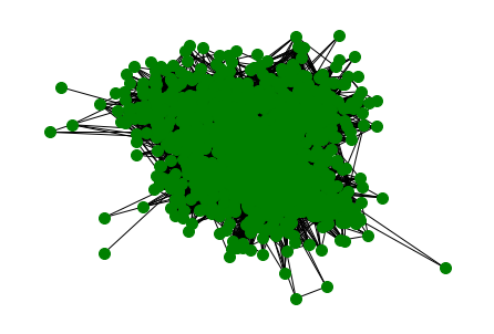
time별 같은 edge 정보를 가지고 있나 확인
np.where(data[0][1].edge_index != data[10][1].edge_index)(array([], dtype=int64), array([], dtype=int64))np.where(data[11][1].edge_index != data[10][1].edge_index)(array([], dtype=int64), array([], dtype=int64))np.where(data[11][1].edge_index != data[20][1].edge_index)(array([], dtype=int64), array([], dtype=int64))https://www.kaggle.com/code/mapologo/loading-wikipedia-math-essentials
from torch_geometric_temporal.dataset import WikiMathsDatasetLoader
loader = WikiMathsDatasetLoader()
dataset = loader.get_dataset(lags=8)
train_dataset, test_dataset = temporal_signal_split(dataset, train_ratio=0.5)data=[]
for time, snapshot in enumerate(train_dataset):
data.append([time,snapshot])(data[0][1]).x[0], (data[0][1]).y[0](tensor([-0.4323, -0.4739, 0.2659, 0.4844, 0.5367, 0.6412, 0.2179, -0.7617]),
tensor(-0.4067))\(t=0\)에서 \(X\)와 \(y\)를 정리하면 아래와 같음.
- X:= \(x_0,x_1,x_2,x_3,,x_4,x_5,x_6,x_7\)
- y:= \(x_9\)
(data[1][1]).x[0],(data[1][1]).y[0](tensor([-0.4739, 0.2659, 0.4844, 0.5367, 0.6412, 0.2179, -0.7617, -0.4067]),
tensor(0.3064))- X:= \(x_1,x_2,x_3,x_4,x_5,x_6,x_7,x_8\)
- y:= \(x_9\)
(data[2][1]).x[0],(data[2][1]).y[0](tensor([ 0.2659, 0.4844, 0.5367, 0.6412, 0.2179, -0.7617, -0.4067, 0.3064]),
tensor(0.4972))- X:=\(x_2,x_3,x_4,x_5,x_6,x_7,x_8,x_9\)
- y:=\(x_{10}\)
하나의 노드에 길이가 \(T\)인 시계열이 맵핑되어 있음. (노드는 총 1068개)
각 노드마다 아래와 같은 과정으로 예측이 됨
- \((x_0,x_1,x_2,x_3,x_4,x_5,x_6,x_7) \to (x_8)\)
- \((x_1,x_2,x_3,x_4,x_5,x_6,x_7,x_8) \to (x_9)\)
\(f(v,t), v \in \{v_1,\dots,v_{1068}\}, t=1,2,\dots,722\)
\[{\bf X}_{t=1} = \begin{bmatrix} f(v_1,t=1) & f(v_1,t=2) & f(v_1,t=3)& f(v_1,t=4) \\ f(v_2,t=1) & f(v_2,t=2) & f(v_2,t=3)& f(v_2,t=4) \\ \dots & \dots & \dots & \dots \\ f(v_{20},t=1) & f(v_{20},t=2) & f(v_{20},t=3)& f(v_{20},t=4) \end{bmatrix}\]
\[{\bf y}_{t=1} = \begin{bmatrix} f(v_1,t=5) \\ f(v_2,t=5) \\ \dots \\ f(v_{20},t=5) \end{bmatrix}\]
Learn
model = RecurrentGCN(node_features=8, filters=32)
optimizer = torch.optim.Adam(model.parameters(), lr=0.01)
model.train()
for epoch in tqdm(range(50)):
for time, snapshot in enumerate(train_dataset):
y_hat = model(snapshot.x, snapshot.edge_index, snapshot.edge_attr)
cost = torch.mean((y_hat-snapshot.y)**2)
cost.backward()
optimizer.step()
optimizer.zero_grad()100%|██████████| 50/50 [09:28<00:00, 11.37s/it]for time, snapshot in enumerate(train_dataset):
_x = snapshot.x
_edge_index = snapshot.edge_index
_edge_attr = snapshot.edge_attr
_y = snapshot.y
break_x.shapetorch.Size([1068, 8])_edge_index.shapetorch.Size([2, 27079])어떤 페이지에 refer가 되었는지
_edge_index[0][:5],_edge_index[1][:5](tensor([0, 0, 0, 0, 0]), tensor([1, 2, 3, 4, 5]))_edge_attr.shapetorch.Size([27079])_edge_attr[:5]tensor([1., 4., 2., 2., 5.])- Weights represent the number of links found at the source Wikipedia page linking to the target Wikipedia page.
가중치는 엣지별 한 페이지에 refer되었는지, 몇 번 되었나 수 나옴
_y.shapetorch.Size([1068])_x.shapetorch.Size([1068, 8])x
- lag 를 몇으로 지정하느냐에 따라 다르게 추출
y
- The target is the daily user visits to the Wikipedia pages between March 16th 2019 and March 15th 2021 which results in 731 periods.
- 매일 위키피디아 해당 페이지에 몇 명의 유저가 방문하는지!
- 음수가 왜 나오지..
_x[0:3]tensor([[-0.4323, -0.4739, 0.2659, 0.4844, 0.5367, 0.6412, 0.2179, -0.7617],
[-0.4041, -0.4165, -0.0751, 0.1484, 0.4153, 0.4464, -0.3916, -0.8137],
[-0.3892, 0.0634, 0.5913, 0.5370, 0.4646, 0.2776, -0.0724, -0.8116]])_y[:3]tensor([-0.4067, -0.1620, -0.4043])y_hat[:3].datatensor([[-0.0648],
[ 0.0314],
[-1.0724]])Windmill Output Datasets
- An hourly windfarm energy output dataset covering 2 years from a European country. Edge weights are calculated from the proximity of the windmills – high weights imply that two windmill stations are in close vicinity. The size of the dataset relates to the groupping of windfarms considered; the smaller datasets are more localized to a single region.
WindmillOutputLargeDatasetLoader
Hourly energy output of windmills from a European country for more than 2 years. Vertices represent 319 windmills and weighted edges describe the strength of relationships. The target variable allows for regression tasks.
데이터정리
- T = 17470
- V = 풍력발전소
- N = 319 # number of nodes
- E = 101761 = N^2 # edges
- \(f(v,t)\)의 차원? (1,) # Hourly energy output
- 시간에 따라서 N이 변하는지? False
- 시간에 따라서 E가 변하는지? False
- X: (319,4) (N,4), \(f(v,t_0),f(v,t_1),f(v,t_2),f(v,t_3)\)
- y: (319,) (N,), \(f(v,t_4)\)
- 예제코드적용가능여부: Yes
- Nodes : 319
- vertices represent 319 windmills
-Edges : 101761
- weighted edges describe the strength of relationships.
- Time : 17470
- more than 2 years
from torch_geometric_temporal.dataset import WindmillOutputLargeDatasetLoader
from torch_geometric_temporal.signal import temporal_signal_split
loader = WindmillOutputLargeDatasetLoader()
dataset = loader.get_dataset(lags=1)
train_dataset, test_dataset = temporal_signal_split(dataset, train_ratio=1)data=[]
for time, snapshot in enumerate(train_dataset):
data.append([time,snapshot])time17470(data[0][1]).x.shape,(data[0][1]).edge_index.shape,(data[0][1]).edge_attr.shape(torch.Size([319, 1]), torch.Size([2, 101761]), torch.Size([101761]))G = nx.Graph()node_list = torch.tensor(range(319)).tolist()G.add_nodes_from(node_list)data[-1][17470, Data(x=[319, 1], edge_index=[2, 101761], edge_attr=[101761], y=[319])]time이 너무 많아서 일부만 시각화함!!
edge_list=[]
for i in range(1000):
for j in range(len(data[0][1].edge_index[0])):
edge_list.append([data[i][1].edge_index[0][j].tolist(),data[i][1].edge_index[1][j].tolist()])G.add_edges_from(edge_list)G.number_of_nodes(),G.number_of_edges()(319, 51040)nx.draw(G,with_labels=True,font_weight='bold',node_color='green',node_size=350,font_color='white',width=1)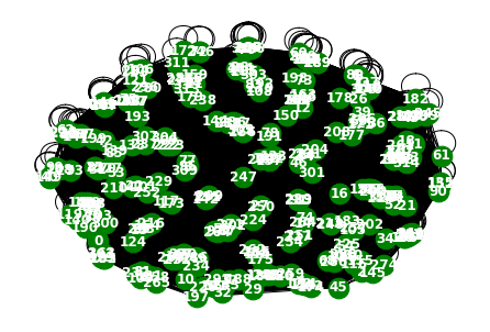
time별 같은 edge 정보를 가지고 있나 확인
np.where(data[0][1].edge_index != data[10][1].edge_index)(array([], dtype=int64), array([], dtype=int64))from torch_geometric_temporal.dataset import WindmillOutputLargeDatasetLoader
loader = WindmillOutputLargeDatasetLoader()
dataset = loader.get_dataset(lags=4)
train_dataset, test_dataset = temporal_signal_split(dataset, train_ratio=0.5)data=[]
for time, snapshot in enumerate(train_dataset):
data.append([time,snapshot])(data[0][1]).x[0], (data[0][1]).y[0](tensor([-0.5711, -0.7560, 2.6278, -0.8674]), tensor(-0.9877))\(t=0\)에서 \(X\)와 \(y\)를 정리하면 아래와 같음.
- X:= \(x_0,x_1,x_2,x_3\)
- y:= \(x_4\)
(data[1][1]).x[0], (data[1][1]).y[0](tensor([-0.7560, 2.6278, -0.8674, -0.9877]), tensor(-0.8583))- X:= \(x_1,x_2,x_3,x_4\)
- y:= \(x_5\)
(data[2][1]).x[0],(data[2][1]).y[0](tensor([ 2.6278, -0.8674, -0.9877, -0.8583]), tensor(0.4282))- X:=\(x_2,x_3,x_4,x_5\)
- y:=\(x_6\)
하나의 노드에 길이가 \(T\)인 시계열이 맵핑되어 있음. (노드는 총 319개)
각 노드마다 아래와 같은 과정으로 예측이 됨
- \((x_0,x_1,x_2,x_3) \to (x_4)\)
- \((x_1,x_2,x_3,x_4) \to (x_5)\)
\(f(v,t), v \in \{v_1,\dots,v_{319}\}, t=1,2,\dots,17470\)
\[{\bf X}_{t=1} = \begin{bmatrix} f(v_1,t=1) & f(v_1,t=2) & f(v_1,t=3)& f(v_1,t=4) \\ f(v_2,t=1) & f(v_2,t=2) & f(v_2,t=3)& f(v_2,t=4) \\ \dots & \dots & \dots & \dots \\ f(v_{20},t=1) & f(v_{20},t=2) & f(v_{20},t=3)& f(v_{20},t=4) \end{bmatrix}\]
\[{\bf y}_{t=1} = \begin{bmatrix} f(v_1,t=5) \\ f(v_2,t=5) \\ \dots \\ f(v_{20},t=5) \end{bmatrix}\]
Learn
model = RecurrentGCN(node_features=4, filters=32)
optimizer = torch.optim.Adam(model.parameters(), lr=0.01)
model.train()
for epoch in tqdm(range(5)):
for time, snapshot in enumerate(train_dataset):
y_hat = model(snapshot.x, snapshot.edge_index, snapshot.edge_attr)
cost = torch.mean((y_hat-snapshot.y)**2)
cost.backward()
optimizer.step()
optimizer.zero_grad()100%|██████████| 5/5 [1:06:03<00:00, 792.70s/it]for time, snapshot in enumerate(train_dataset):
_x = snapshot.x
_edge_index = snapshot.edge_index
_edge_attr = snapshot.edge_attr
_y = snapshot.y
break_x.shapetorch.Size([319, 4])_edge_index.shapetorch.Size([2, 101761])_edge_attr.shapetorch.Size([101761])_y.shapetorch.Size([319])_x.shapetorch.Size([319, 4])x
y
- The target variable allows for regression tasks.
_x[0:3]tensor([[-0.5711, -0.7560, 2.6278, -0.8674],
[-0.6936, -0.7264, 2.4113, -0.6052],
[-0.8666, -0.7785, 2.2759, -0.6759]])_y[0]tensor(-0.9877)WindmillOutputMediumDatasetLoader
Hourly energy output of windmills from a European country for more than 2 years. Vertices represent 26 windmills and weighted edges describe the strength of relationships. The target variable allows for regression tasks.
데이터정리
- T = 17470
- V = 풍력발전소
- N = 319 # number of nodes
- E = 101761 = N^2 # edges
- \(f(v,t)\)의 차원? (1,) # Hourly energy output
- 시간에 따라서 N이 변하는지? False
- 시간에 따라서 E가 변하는지? False
- X: (319,4) (N,4), \(f(v,t_0),f(v,t_1),f(v,t_2),f(v,t_3)\)
- y: (319,) (N,), \(f(v,t_4)\)
- 예제코드적용가능여부: Yes
- Nodes : 26
- vertices represent 26 windmills
-Edges : 225
- weighted edges describe the strength of relationships
- Time : 676
- more than 2 years
from torch_geometric_temporal.dataset import WindmillOutputMediumDatasetLoader
from torch_geometric_temporal.signal import temporal_signal_split
loader = WindmillOutputMediumDatasetLoader()
dataset = loader.get_dataset(lags=1)
train_dataset, test_dataset = temporal_signal_split(dataset, train_ratio=1)data=[]
for time, snapshot in enumerate(train_dataset):
data.append([time,snapshot])time17470(data[0][1]).x.shape,(data[0][1]).edge_index.shape,(data[0][1]).edge_attr.shape(torch.Size([26, 1]), torch.Size([2, 676]), torch.Size([676]))G = nx.Graph()node_list = torch.tensor(range(26)).tolist()G.add_nodes_from(node_list)data[-1][17470, Data(x=[26, 1], edge_index=[2, 676], edge_attr=[676], y=[26])]edge_list=[]
for i in range(17463):
for j in range(len(data[0][1].edge_index[0])):
edge_list.append([data[i][1].edge_index[0][j].tolist(),data[i][1].edge_index[1][j].tolist()])G.add_edges_from(edge_list)G.number_of_nodes(),G.number_of_edges()(26, 351)nx.draw(G,with_labels=True,font_weight='bold',node_color='green',node_size=350,font_color='white',width=1)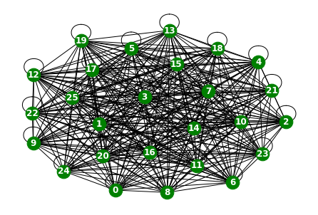
time별 같은 edge 정보를 가지고 있나 확인
np.where(data[0][1].edge_index != data[10][1].edge_index)(array([], dtype=int64), array([], dtype=int64))from torch_geometric_temporal.dataset import WindmillOutputMediumDatasetLoader
loader = WindmillOutputMediumDatasetLoader()
dataset = loader.get_dataset(lags=4)
train_dataset, test_dataset = temporal_signal_split(dataset, train_ratio=0.5)data=[]
for time, snapshot in enumerate(train_dataset):
data.append([time,snapshot])(data[0][1]).x[0], (data[0][1]).y[0](tensor([-0.2170, -0.2055, -0.1587, -0.1930]), tensor(-0.2149))\(t=0\)에서 \(X\)와 \(y\)를 정리하면 아래와 같음.
- X:= \(x_0,x_1,x_2,x_3\)
- y:= \(x_4\)
(data[1][1]).x[0],(data[1][1]).y[0](tensor([-0.2055, -0.1587, -0.1930, -0.2149]), tensor(-0.2336))- X:= \(x_1,x_2,x_3,x_4\)
- y:= \(x_5\)
(data[2][1]).x[0],(data[2][1]).y[0](tensor([-0.1587, -0.1930, -0.2149, -0.2336]), tensor(-0.1785))- X:=\(x_2,x_3,x_4,x_5\)
- y:=\(x_6\)
하나의 노드에 길이가 \(T\)인 시계열이 맵핑되어 있음. (노드는 총 26개)
각 노드마다 아래와 같은 과정으로 예측이 됨
- \((x_0,x_1,x_2,x_3) \to (x_4)\)
- \((x_1,x_2,x_3,x_4) \to (x_5)\)
\(f(v,t), v \in \{v_1,\dots,v_{26}\}, t=1,2,\dots,177470\)
\[{\bf X}_{t=1} = \begin{bmatrix} f(v_1,t=1) & f(v_1,t=2) & f(v_1,t=3)& f(v_1,t=4) \\ f(v_2,t=1) & f(v_2,t=2) & f(v_2,t=3)& f(v_2,t=4) \\ \dots & \dots & \dots & \dots \\ f(v_{20},t=1) & f(v_{20},t=2) & f(v_{20},t=3)& f(v_{20},t=4) \end{bmatrix}\]
\[{\bf y}_{t=1} = \begin{bmatrix} f(v_1,t=5) \\ f(v_2,t=5) \\ \dots \\ f(v_{20},t=5) \end{bmatrix}\]
Learn
model = RecurrentGCN(node_features=4, filters=32)
optimizer = torch.optim.Adam(model.parameters(), lr=0.01)
model.train()
for epoch in tqdm(range(5)):
for time, snapshot in enumerate(train_dataset):
y_hat = model(snapshot.x, snapshot.edge_index, snapshot.edge_attr)
cost = torch.mean((y_hat-snapshot.y)**2)
cost.backward()
optimizer.step()
optimizer.zero_grad()100%|██████████| 5/5 [03:23<00:00, 40.73s/it]for time, snapshot in enumerate(train_dataset):
_x = snapshot.x
_edge_index = snapshot.edge_index
_edge_attr = snapshot.edge_attr
_y = snapshot.y
break_x.shapetorch.Size([26, 4])_edge_index.shapetorch.Size([2, 676])_edge_attr.shapetorch.Size([676])_y.shapetorch.Size([26])_x.shapetorch.Size([26, 4])x
y
- The target variable allows for regression tasks.
_x[0:3]tensor([[-0.2170, -0.2055, -0.1587, -0.1930],
[-0.1682, -0.2708, -0.1051, 1.1786],
[ 1.1540, -0.6707, -0.8291, -0.6823]])_y[0]tensor(-0.2149)WindmillOutputSmallDatasetLoader
Hourly energy output of windmills from a European country for more than 2 years. Vertices represent 11 windmills and weighted edges describe the strength of relationships. The target variable allows for regression tasks.
데이터정리
- T = 17470
- V = 풍력발전소
- N = 11 # number of nodes
- E = 121 = N^2 # edges
- \(f(v,t)\)의 차원? (1,) # Hourly energy output
- 시간에 따라서 N이 변하는지? False
- 시간에 따라서 E가 변하는지? False
- X: (11,4) (N,4), \(f(v,t_0),f(v,t_1),f(v,t_2),f(v,t_3)\)
- y: (11,) (N,), \(f(v,t_4)\)
- 예제코드적용가능여부: Yes
- Nodes : 11
- vertices represent 11 windmills
-Edges : 121
- weighted edges describe the strength of relationships
- Time : 17470
- more than 2 years
from torch_geometric_temporal.dataset import WindmillOutputSmallDatasetLoader
from torch_geometric_temporal.signal import temporal_signal_split
loader = WindmillOutputSmallDatasetLoader()
dataset = loader.get_dataset()
train_dataset, test_dataset = temporal_signal_split(dataset, train_ratio=1)data=[]
for time, snapshot in enumerate(train_dataset):
data.append([time,snapshot])time17463(data[0][1]).x.shape,(data[0][1]).edge_index.shape,(data[0][1]).edge_attr.shape(torch.Size([11, 8]), torch.Size([2, 121]), torch.Size([121]))data[-1][17463, Data(x=[11, 8], edge_index=[2, 121], edge_attr=[121], y=[11])]G = nx.Graph()node_list = torch.tensor(range(11)).tolist()G.add_nodes_from(node_list)edge_list=[]
for i in range(17463):
for j in range(len(data[0][1].edge_index[0])):
edge_list.append([data[i][1].edge_index[0][j].tolist(),data[i][1].edge_index[1][j].tolist()])G.add_edges_from(edge_list)G.number_of_nodes(),G.number_of_edges()(11, 66)nx.draw(G,with_labels=True,font_weight='bold',node_color='green',node_size=350,font_color='white',width=1)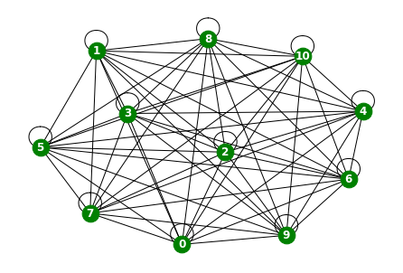
time별 같은 edge 정보를 가지고 있나 확인
np.where(data[0][1].edge_index != data[10][1].edge_index)(array([], dtype=int64), array([], dtype=int64))from torch_geometric_temporal.dataset import WindmillOutputSmallDatasetLoader
loader = WindmillOutputSmallDatasetLoader()
dataset = loader.get_dataset(lags=4)
train_dataset, test_dataset = temporal_signal_split(dataset, train_ratio=0.5)data=[]
for time, snapshot in enumerate(train_dataset):
data.append([time,snapshot])(data[0][1]).x[0], (data[0][1]).y[0](tensor([ 0.8199, -0.4972, 0.4923, -0.8299]), tensor(-0.6885))\(t=0\)에서 \(X\)와 \(y\)를 정리하면 아래와 같음.
- X:= \(x_0,x_1,x_2,x_3\)
- y:= \(x_4\)
(data[1][1]).x[0],(data[1][1]).y[0](tensor([-0.4972, 0.4923, -0.8299, -0.6885]), tensor(0.7092))- X:= \(x_1,x_2,x_3,x_4\)
- y:= \(x_5\)
(data[2][1]).x[0],(data[2][1]).y[0](tensor([ 0.4923, -0.8299, -0.6885, 0.7092]), tensor(-0.9356))- X:=\(x_2,x_3,x_4,x_5\)
- y:=\(x_6\)
하나의 노드에 길이가 \(T\)인 시계열이 맵핑되어 있음. (노드는 총 11개)
각 노드마다 아래와 같은 과정으로 예측이 됨
- \((x_0,x_1,x_2,x_3) \to (x_4)\)
- \((x_1,x_2,x_3,x_4) \to (x_5)\)
\(f(v,t), v \in \{v_1,\dots,v_{11}\}, t=1,2,\dots,17463\)
\[{\bf X}_{t=1} = \begin{bmatrix} f(v_1,t=1) & f(v_1,t=2) & f(v_1,t=3)& f(v_1,t=4) \\ f(v_2,t=1) & f(v_2,t=2) & f(v_2,t=3)& f(v_2,t=4) \\ \dots & \dots & \dots & \dots \\ f(v_{20},t=1) & f(v_{20},t=2) & f(v_{20},t=3)& f(v_{20},t=4) \end{bmatrix}\]
\[{\bf y}_{t=1} = \begin{bmatrix} f(v_1,t=5) \\ f(v_2,t=5) \\ \dots \\ f(v_{20},t=5) \end{bmatrix}\]
Learn
model = RecurrentGCN(node_features=4, filters=32)
optimizer = torch.optim.Adam(model.parameters(), lr=0.01)
model.train()
for epoch in tqdm(range(5)):
for time, snapshot in enumerate(train_dataset):
y_hat = model(snapshot.x, snapshot.edge_index, snapshot.edge_attr)
cost = torch.mean((y_hat-snapshot.y)**2)
cost.backward()
optimizer.step()
optimizer.zero_grad()100%|██████████| 5/5 [02:55<00:00, 35.01s/it]for time, snapshot in enumerate(train_dataset):
_x = snapshot.x
_edge_index = snapshot.edge_index
_edge_attr = snapshot.edge_attr
_y = snapshot.y
break_x.shapetorch.Size([11, 4])_edge_index.shapetorch.Size([2, 121])_edge_attr.shapetorch.Size([121])_y.shapetorch.Size([11])_x.shapetorch.Size([11, 4])x
y
- The target variable allows for regression tasks.
_x[0:3]tensor([[ 0.8199, -0.4972, 0.4923, -0.8299],
[ 1.1377, -0.3742, 0.3668, -0.8333],
[ 0.9979, -0.5643, 0.4070, -0.8918]])_ytensor([-0.6885, -0.6594, -0.6303, -0.6983, -0.5416, -0.6186, -0.6031, -0.7580,
-0.6659, -0.5948, -0.5088])METRLADatasetLoader_real world traffic dataset
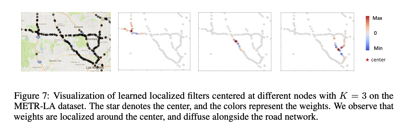
A traffic forecasting dataset based on Los Angeles Metropolitan traffic conditions. The dataset contains traffic readings collected from 207 loop detectors on highways in Los Angeles County in aggregated 5 minute intervals for 4 months between March 2012 to June 2012.
데이터정리
- T = 33
- V = 구역
- N = 207 # number of nodes
- E = 225
- \(f(v,t)\)의 차원? (3,) # Hourly energy output
- 시간에 따라서 N이 변하는지? False
- 시간에 따라서 E가 변하는지? False
- X: (207,4) (N,2,12), \(x_0,x_1,x_2,x_3,x_4,x_5,x_6,x_7,x_8,x_9,x_{10},x_{11},z_0,z_1,z_2,z_3,z_4,z_5,z_6,z_7,z_8,z_9,z_{10},z_{11}\)
- y: (207,) (N,), \((x_{12})\)
- 예제코드적용가능여부: No
https://arxiv.org/pdf/1707.01926.pdf
- Nodes : 207
- vertices are localities
-Edges : 225
- edges are spatial_connections
- Time : 33
- between 2020 and 2021
- per weeks
from torch_geometric_temporal.dataset import METRLADatasetLoader
from torch_geometric_temporal.signal import temporal_signal_split
loader = METRLADatasetLoader()
dataset = loader.get_dataset()
train_dataset, test_dataset = temporal_signal_split(dataset, train_ratio=1)data=[]
for time, snapshot in enumerate(train_dataset):
data.append([time,snapshot])time34248(data[0][1]).x.shape,(data[0][1]).edge_index.shape,(data[0][1]).edge_attr.shape(torch.Size([207, 2, 12]), torch.Size([2, 1722]), torch.Size([1722]))data[-1][34248,
Data(x=[207, 2, 12], edge_index=[2, 1722], edge_attr=[1722], y=[207, 12])]G = nx.Graph()node_list = torch.tensor(range(20)).tolist()G.add_nodes_from(node_list)edge_list=[]
for i in range(1000):
for j in range(len(data[0][1].edge_index[0])):
edge_list.append([data[i][1].edge_index[0][j].tolist(),data[i][1].edge_index[1][j].tolist()])G.add_edges_from(edge_list)G.number_of_nodes(),G.number_of_edges()(207, 1520)nx.draw(G,with_labels=True,font_weight='bold',node_color='green',node_size=350,font_color='white',width=1)
time별 같은 edge 정보를 가지고 있나 확인
np.where(data[0][1].edge_index != data[10][1].edge_index)(array([], dtype=int64), array([], dtype=int64))논문 내용 중
from torch_geometric_temporal.dataset import METRLADatasetLoader
loader = METRLADatasetLoader()
dataset = loader.get_dataset()
train_dataset, test_dataset = temporal_signal_split(dataset, train_ratio=0.5)
Note
lags option 없어서 error 뜸 : get_dataset() got an unexpected keyword argument ‘lags’
data=[]
for time, snapshot in enumerate(train_dataset):
data.append([time,snapshot])(data[0][1]).x[0], (data[0][1]).y[0](tensor([[ 0.5332, 0.4486, 0.5146, -2.6522, -2.6522, 0.1847, 0.6383, 0.4961,
0.7497, 0.4899, 0.5751, 0.4280],
[-1.7292, -1.7171, -1.7051, -1.6930, -1.6810, -1.6689, -1.6569, -1.6448,
-1.6328, -1.6207, -1.6087, -1.5966]]),
tensor([0.3724, 0.2452, 0.4961, 0.6521, 0.1126, 0.5311, 0.5091, 0.4713, 0.4218,
0.3909, 0.4761, 0.5641]))\(t=0\)에서 \(X,Z\)와 \(y\)를 정리하면 아래와 같음.
- X:= \(x_0,x_1,x_2,x_3,x_4,x_5,x_6,x_7,x_8,x_9,x_{10},x_{11}\)
- Z:= \(z_0,z_1,z_2,z_3,z_4,z_5,z_6,z_7,z_8,z_9,z_{10},z_{11}\)
- y:= \(x_{12}\)
(data[1][1]).x[0],(data[1][1]).y[0](tensor([[ 0.4486, 0.5146, -2.6522, -2.6522, 0.1847, 0.6383, 0.4961, 0.7497,
0.4899, 0.5751, 0.4280, 0.3724],
[-1.7171, -1.7051, -1.6930, -1.6810, -1.6689, -1.6569, -1.6448, -1.6328,
-1.6207, -1.6087, -1.5966, -1.5846]]),
tensor([ 0.2452, 0.4961, 0.6521, 0.1126, 0.5311, 0.5091, 0.4713, 0.4218,
0.3909, 0.4761, 0.5641, -0.0022]))- X:= \(x_1,x_2,x_3,x_4,x_5,x_6,x_7,x_8,x_9,x_{10},x_{11},x_{12}\)
- Z:= \(z_1,z_2,z_3,z_4,z_5,z_6,z_7,z_8,z_9,z_{10},z_{11},z_{12}\)
- y:= \(x_{13}\)
(data[2][1]).x[0],(data[2][1]).y[0](tensor([[ 0.5146, -2.6522, -2.6522, 0.1847, 0.6383, 0.4961, 0.7497, 0.4899,
0.5751, 0.4280, 0.3724, 0.2452],
[-1.7051, -1.6930, -1.6810, -1.6689, -1.6569, -1.6448, -1.6328, -1.6207,
-1.6087, -1.5966, -1.5846, -1.5725]]),
tensor([ 0.4961, 0.6521, 0.1126, 0.5311, 0.5091, 0.4713, 0.4218, 0.3909,
0.4761, 0.5641, -0.0022, 0.4218]))- X:= \(x_2,x_3,x_4,x_5,x_6,x_7,x_8,x_9,x_{10},x_{11},x_{12},x_{13}\)
- Z:= \(z_2,z_3,z_4,z_5,z_6,z_7,z_8,z_9,z_{10},z_{11},z_{12},z_{13}\)
- y:= \(x_{14}\)
하나의 노드에 길이가 \(T\)인 시계열이 맵핑되어 있음. (노드는 총 207개)
각 노드마다 아래와 같은 과정으로 예측이 됨
- \(x_0,x_1,x_2,x_3,x_4,x_5,x_6,x_7,x_8,x_9,x_{10},x_{11},z_0,z_1,z_2,z_3,z_4,z_5,z_6,z_7,z_8,z_9,z_{10},z_{11} \to (x_{12})\)
- \(x_1,x_2,x_3,x_4,x_5,x_6,x_7,x_8,x_9,x_{10},x_{11},x_{12},z_1,z_2,z_3,z_4,z_5,z_6,z_7,z_8,z_9,z_{10},z_{11},z_{12} \to (x_{13})\)
\(f(v,t), v \in \{v_1,\dots,v_{207}\}, t=1,2,\dots,34248\)
\[{\bf X}_{t=1} = \begin{bmatrix} f(v_1,t=1) & f(v_1,t=2) & f(v_1,t=3)& f(v_1,t=4) \\ f(v_2,t=1) & f(v_2,t=2) & f(v_2,t=3)& f(v_2,t=4) \\ \dots & \dots & \dots & \dots \\ f(v_{20},t=1) & f(v_{20},t=2) & f(v_{20},t=3)& f(v_{20},t=4) \end{bmatrix}\]
\[{\bf y}_{t=1} = \begin{bmatrix} f(v_1,t=5) \\ f(v_2,t=5) \\ \dots \\ f(v_{20},t=5) \end{bmatrix}\]
Learn
model = RecurrentGCN(node_features=1, filters=32)
optimizer = torch.optim.Adam(model.parameters(), lr=0.01)
model.train()
for epoch in tqdm(range(50)):
for time, snapshot in enumerate(train_dataset):
y_hat = model(snapshot.x, snapshot.edge_index, snapshot.edge_attr)
cost = torch.mean((y_hat-snapshot.y)**2)
cost.backward()
optimizer.step()
optimizer.zero_grad()for time, snapshot in enumerate(train_dataset):
_x = snapshot.x
_edge_index = snapshot.edge_index
_edge_attr = snapshot.edge_attr
_y = snapshot.y
break_x.shapetorch.Size([207, 2, 12])- node 207개, traffic sensor 2개
_edge_index.shapetorch.Size([2, 1722])_edge_attr.shapetorch.Size([1722])_y.shapetorch.Size([207, 12])_x.shapetorch.Size([207, 2, 12])y
- traffic speed
_x[0]tensor([[ 0.5332, 0.4486, 0.5146, -2.6522, -2.6522, 0.1847, 0.6383, 0.4961,
0.7497, 0.4899, 0.5751, 0.4280],
[-1.7292, -1.7171, -1.7051, -1.6930, -1.6810, -1.6689, -1.6569, -1.6448,
-1.6328, -1.6207, -1.6087, -1.5966]])_y[0]tensor([0.3724, 0.2452, 0.4961, 0.6521, 0.1126, 0.5311, 0.5091, 0.4713, 0.4218,
0.3909, 0.4761, 0.5641])PemsBayDatasetLoader
https://onlinelibrary.wiley.com/doi/pdf/10.1111/tgis.12644
A traffic forecasting dataset as described in Diffusion Convolution Layer Paper.
This traffic dataset is collected by California Transportation Agencies (CalTrans) Performance Measurement System (PeMS). It is represented by a network of 325 traffic sensors in the Bay Area with 6 months of traffic readings ranging from Jan 1st 2017 to May 31th 2017 in 5 minute intervals.
데이터정리
- T = 17470
- V = 풍력발전소
- N = 325 # number of nodes
- E = 101761 = N^2 # edges
- \(f(v,t)\)의 차원? (1,) # Hourly energy output
- 시간에 따라서 N이 변하는지? False
- 시간에 따라서 E가 변하는지? False
- X: (325,2,12) (N,2,12),
- \(x_0,x_1,x_2,x_3,x_4,x_5,x_6,x_7,x_8,x_9,x_{10},x_{11}\)
- \(z_0,z_1,z_2,z_3,z_4,z_5,z_6,z_7,z_8,z_9,z_{10},z_{11}\)
- y: (325,) (N,2,12),
- \(x_{13},x_{14},x_{15},x_{16},x_{17},x_{18},x_{19},x_{20},x_{21},x_{22},x_{23},x_{24}\)
- \(z_{13},z_{14},z_{15},z_{16},z_{17},z_{18},z_{19},z_{20},z_{21},z_{22},z_{23},z_{24}\)
- 예제코드적용가능여부: No
- Nodes : 325
- vertices are sensors
-Edges : 2694
- weighted edges are between seonsor paris measured by the road nretwork distance
- Time : 52081
- 6 months of traffic readings ranging from Jan 1st 2017 to May 31th 2017 in 5 minute intervals
from torch_geometric_temporal.dataset import PemsBayDatasetLoader
from torch_geometric_temporal.signal import temporal_signal_split
loader = PemsBayDatasetLoader()
dataset = loader.get_dataset()
train_dataset, test_dataset = temporal_signal_split(dataset, train_ratio=1)data=[]
for time, snapshot in enumerate(train_dataset):
data.append([time,snapshot])time52081(data[0][1]).x.shape,(data[0][1]).edge_index.shape,(data[0][1]).edge_attr.shape(torch.Size([325, 2, 12]), torch.Size([2, 2694]), torch.Size([2694]))G = nx.Graph()node_list = torch.tensor(range(325)).tolist()data[-1][52081,
Data(x=[325, 2, 12], edge_index=[2, 2694], edge_attr=[2694], y=[325, 2, 12])]G.add_nodes_from(node_list)edge_list=[]
for i in range(1000):
for j in range(len(data[0][1].edge_index[0])):
edge_list.append([data[i][1].edge_index[0][j].tolist(),data[i][1].edge_index[1][j].tolist()])G.add_edges_from(edge_list)G.number_of_nodes(),G.number_of_edges()(325, 2404)nx.draw(G,node_color='green',node_size=50,font_color='white',width=1)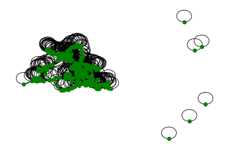
time별 같은 edge 정보를 가지고 있나 확인
np.where(data[0][1].edge_index != data[10][1].edge_index)(array([], dtype=int64), array([], dtype=int64))from torch_geometric_temporal.dataset import PemsBayDatasetLoader
loader = PemsBayDatasetLoader()
dataset = loader.get_dataset()
train_dataset, test_dataset = temporal_signal_split(dataset, train_ratio=0.5)data=[]
for time, snapshot in enumerate(train_dataset):
data.append([time,snapshot])(data[0][1]).x[0], (data[0][1]).y[0](tensor([[ 0.9821, 0.9928, 1.0251, 1.0574, 1.0466, 1.0681, 0.9821, 1.0251,
1.0143, 0.9928, 0.9498, 0.9821],
[-1.6127, -1.6005, -1.5883, -1.5762, -1.5640, -1.5518, -1.5397, -1.5275,
-1.5153, -1.5032, -1.4910, -1.4788]]),
tensor([[ 1.0143, 0.9821, 0.9821, 1.0036, 1.0143, 0.9605, 0.9498, 1.0251,
0.9928, 0.9928, 0.9498, 0.9928],
[-1.4667, -1.4545, -1.4423, -1.4302, -1.4180, -1.4058, -1.3937, -1.3815,
-1.3694, -1.3572, -1.3450, -1.3329]]))\(t=0\)에서 \(X,Z\)와 \(y,s\)를 정리하면 아래와 같음.
- X:= \(x_0,x_1,x_2,x_3,x_4,x_5,x_6,x_7,x_8,x_9,x_{10},x_{11}\)
- Z:= \(z_0,z_1,z_2,z_3,z_4,z_5,z_6,z_7,z_8,z_9,z_{10},z_{11}\)
- y:= \(x_{12},x_{13},x_{14},x_{15},x_{16},x_{17},x_{18},x_{19},x_{20},x_{21},x_{22},x_{23}\)
- s:= \(z_{12},z_{13},z_{14},z_{15},z_{16},z_{17},z_{18},z_{19},z_{20},z_{21},z_{22},z_{23}\)
(data[1][1]).x[0],(data[1][1]).y[0](tensor([[ 0.9928, 1.0251, 1.0574, 1.0466, 1.0681, 0.9821, 1.0251, 1.0143,
0.9928, 0.9498, 0.9821, 1.0143],
[-1.6005, -1.5883, -1.5762, -1.5640, -1.5518, -1.5397, -1.5275, -1.5153,
-1.5032, -1.4910, -1.4788, -1.4667]]),
tensor([[ 0.9821, 0.9821, 1.0036, 1.0143, 0.9605, 0.9498, 1.0251, 0.9928,
0.9928, 0.9498, 0.9928, 0.9821],
[-1.4545, -1.4423, -1.4302, -1.4180, -1.4058, -1.3937, -1.3815, -1.3694,
-1.3572, -1.3450, -1.3329, -1.3207]]))- X:= \(x_1,x_2,x_3,x_4,x_5,x_6,x_7,x_8,x_9,x_{10},x_{11},x_{12}\)
- Z:= \(z_1,z_2,z_3,z_4,z_5,z_6,z_7,z_8,z_9,z_{10},z_{11},z_{12}\)
- y:= \(x_{13},x_{14},x_{15},x_{16},x_{17},x_{18},x_{19},x_{20},x_{21},x_{22},x_{23},x_{24}\)
- s:= \(z_{13},z_{14},z_{15},z_{16},z_{17},z_{18},z_{19},z_{20},z_{21},z_{22},z_{23},z_{24}\)
(data[2][1]).x[0],(data[2][1]).y[0](tensor([[ 1.0251, 1.0574, 1.0466, 1.0681, 0.9821, 1.0251, 1.0143, 0.9928,
0.9498, 0.9821, 1.0143, 0.9821],
[-1.5883, -1.5762, -1.5640, -1.5518, -1.5397, -1.5275, -1.5153, -1.5032,
-1.4910, -1.4788, -1.4667, -1.4545]]),
tensor([[ 0.9821, 1.0036, 1.0143, 0.9605, 0.9498, 1.0251, 0.9928, 0.9928,
0.9498, 0.9928, 0.9821, 1.0143],
[-1.4423, -1.4302, -1.4180, -1.4058, -1.3937, -1.3815, -1.3694, -1.3572,
-1.3450, -1.3329, -1.3207, -1.3085]]))- X:= \(x_2,x_3,x_4,x_5,x_6,x_7,x_8,x_9,x_{10},x_{11},x_{12},x_{13}\)
- Z:= \(z_2,z_3,z_4,z_5,z_6,z_7,z_8,z_9,z_{10},z_{11},z_{12},z_{13}\)
- y:= \(x_{14},x_{15},x_{16},x_{17},x_{18},x_{19},x_{20},x_{21},x_{22},x_{23},x_{24},x_{25}\)
- s:= \(z_{14},z_{15},z_{16},z_{17},z_{18},z_{19},z_{20},z_{21},z_{22},z_{23},z_{24},z_{25}\)
하나의 노드에 길이가 \(T\)인 시계열이 맵핑되어 있음. (노드는 총 325개)
각 노드마다 아래와 같은 과정으로 예측이 됨
- \(x_0,x_1,x_2,x_3,x_4,x_5,x_6,x_7,x_8,x_9,x_{10},x_{11} \to x_{12},x_{13},x_{14},x_{15},x_{16},x_{17},x_{18},x_{19},x_{20},x_{21},x_{22},x_{23}\)
- \(z_0,z_1,z_2,z_3,z_4,z_5,z_6,z_7,z_8,z_9,z_{10},z_{11} \to z_{12},z_{13},z_{14},z_{15},z_{16},z_{17},z_{18},z_{19},z_{20},z_{21},z_{22},z_{23}\)
- \(x_1,x_2,x_3,x_4,x_5,x_6,x_7,x_8,x_9,x_{10},x_{11},x_{12} \to x_{13},x_{14},x_{15},x_{16},x_{17},x_{18},x_{19},x_{20},x_{21},x_{22},x_{23},x_{24}\)
- \(z_1,z_2,z_3,z_4,z_5,z_6,z_7,z_8,z_9,z_{10},z_{11},z_{12} \to z_{13},z_{14},z_{15},z_{16},z_{17},z_{18},z_{19},z_{20},z_{21},z_{22},z_{23},z_{24}\)
\(f(v,t), v \in \{v_1,\dots,v_{325}\}, t=1,2,\dots,52081\)
\[{\bf X}_{t=1} = \begin{bmatrix} f(v_1,t=1) & f(v_1,t=2) & f(v_1,t=3)& f(v_1,t=4) \\ f(v_2,t=1) & f(v_2,t=2) & f(v_2,t=3)& f(v_2,t=4) \\ \dots & \dots & \dots & \dots \\ f(v_{20},t=1) & f(v_{20},t=2) & f(v_{20},t=3)& f(v_{20},t=4) \end{bmatrix}\]
\[{\bf y}_{t=1} = \begin{bmatrix} f(v_1,t=5) \\ f(v_2,t=5) \\ \dots \\ f(v_{20},t=5) \end{bmatrix}\]
Learn
model = RecurrentGCN(node_features=4, filters=32)

optimizer = torch.optim.Adam(model.parameters(), lr=0.01)

model.train()

for epoch in tqdm(range(50)):
    for time, snapshot in enumerate(train_dataset):
        y_hat = model(snapshot.x, snapshot.edge_index, snapshot.edge_attr)
        cost = torch.mean((y_hat-snapshot.y)**2)
        cost.backward()
        optimizer.step()
optimizer.zero_grad()for time, snapshot in enumerate(train_dataset):
_x = snapshot.x
_edge_index = snapshot.edge_index
_edge_attr = snapshot.edge_attr
_y = snapshot.y
break_x.shapetorch.Size([325, 2, 12])_edge_index.shapetorch.Size([2, 2694])_edge_attr.shapetorch.Size([2694])_y.shapetorch.Size([325, 2, 12])_x.shapetorch.Size([325, 2, 12])x
- .!
y
- capturing temporal dependencies..?
edges connect sensors
For instance, the traffic conditions on one road on Wednesday at 3:00 p.m. are similar to the traffic conditions on Thursday at the same time.
_x[0:3]tensor([[[ 0.9821, 0.9928, 1.0251, 1.0574, 1.0466, 1.0681, 0.9821,
1.0251, 1.0143, 0.9928, 0.9498, 0.9821],
[-1.6127, -1.6005, -1.5883, -1.5762, -1.5640, -1.5518, -1.5397,
-1.5275, -1.5153, -1.5032, -1.4910, -1.4788]],
[[ 0.6054, 0.5839, 0.6592, 0.6269, 0.6808, 0.6377, 0.6700,
0.6054, 0.6162, 0.6162, 0.5839, 0.5947],
[-1.6127, -1.6005, -1.5883, -1.5762, -1.5640, -1.5518, -1.5397,
-1.5275, -1.5153, -1.5032, -1.4910, -1.4788]],
[[ 0.9390, 0.9175, 0.8960, 0.9175, 0.9067, 0.9175, 0.9175,
0.8852, 0.9283, 0.8960, 0.9067, 0.8960],
[-1.6127, -1.6005, -1.5883, -1.5762, -1.5640, -1.5518, -1.5397,
-1.5275, -1.5153, -1.5032, -1.4910, -1.4788]]])_y[0]tensor([[ 1.0143, 0.9821, 0.9821, 1.0036, 1.0143, 0.9605, 0.9498, 1.0251,
0.9928, 0.9928, 0.9498, 0.9928],
[-1.4667, -1.4545, -1.4423, -1.4302, -1.4180, -1.4058, -1.3937, -1.3815,
-1.3694, -1.3572, -1.3450, -1.3329]])EnglandCovidDatasetLoader
Covid19 England
- A dataset about mass mobility between regions in England and the number of confirmed COVID-19 cases from March to May 2020 [38]. Each day contains a different mobility graph and node features corresponding to the number of cases in the previous days. Mobility stems from Facebook Data For Good 1 and cases from gov.uk 2
https://arxiv.org/pdf/2009.08388.pdf
데이터정리
- T = 52
- V = 지역
- N = 129 # number of nodes
- E = 2158
- \(f(v,t)\)의 차원? (1,) # 코로나확진자수
- 시간에 따라서 Number of nodes가 변하는지? False
- 시간에 따라서 Number of nodes가 변하는지? False
- X: (20,4) (N,4), \(f(v,t_0),f(v,t_1),f(v,t_2),f(v,t_3)\)
- y: (20,) (N,), \(f(v,t_4)\)
- 예제코드적용가능여부: Yes
- Nodes : 129
- vertices are correspond to the number of COVID-19 cases in the region in the past window days.
-Edges : 2158
- the spatial edges capture county-to-county movement at a specific date, and a county is connected to a number of past instances of itself with temporal edges.
- Time : 52
- from 3 March to 12 of May
from torch_geometric_temporal.dataset import EnglandCovidDatasetLoader
from torch_geometric_temporal.signal import temporal_signal_split
loader = EnglandCovidDatasetLoader()
dataset = loader.get_dataset()
train_dataset, test_dataset = temporal_signal_split(dataset, train_ratio=1)data=[]
for time, snapshot in enumerate(train_dataset):
data.append([time,snapshot])time52(data[0][1]).x.shape,(data[0][1]).edge_index.shape,(data[0][1]).edge_attr.shape(torch.Size([129, 8]), torch.Size([2, 2158]), torch.Size([2158]))G = nx.Graph()node_list = torch.tensor(range(129)).tolist()G.add_nodes_from(node_list)data[-1][52, Data(x=[129, 8], edge_index=[2, 1424], edge_attr=[1424], y=[129])]len(data[0][1].edge_index[0])2158edge_list=[]
for i in range(52):
for j in range(100):
edge_list.append([data[i][1].edge_index[0][j].tolist(),data[i][1].edge_index[1][j].tolist()])G.add_edges_from(edge_list)G.number_of_nodes(),G.number_of_edges()(129, 1230)nx.draw(G,with_labels=True,font_weight='bold',node_color='green',node_size=350,font_color='white',width=1)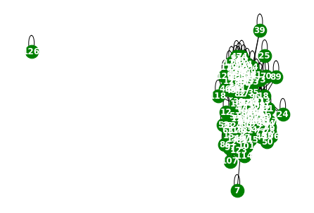
time별 같은 edge 정보를 가지고 있나 확인
np.where(data[2][1].edge_index !=data[2][1].edge_index)(array([], dtype=int64), array([], dtype=int64))from torch_geometric_temporal.dataset import EnglandCovidDatasetLoader
loader = EnglandCovidDatasetLoader()
dataset = loader.get_dataset(lags=4)
train_dataset, test_dataset = temporal_signal_split(dataset, train_ratio=0.5)data=[]
for time, snapshot in enumerate(train_dataset):
data.append([time,snapshot])(data[0][1]).x[0], (data[0][1]).y[0](tensor([-1.4697, -1.9283, -1.6990, -1.8137]), tensor(-1.8137))\(t=0\)에서 \(X\)와 \(y\)를 정리하면 아래와 같음.
- X:= \(x_0,x_1,x_2,x_3\)
- y:= \(x_4\)
(data[1][1]).x[0],(data[1][1]).y[0](tensor([-1.9283, -1.6990, -1.8137, -1.8137]), tensor(-0.8965))- X:= \(x_1,x_2,x_3,x_4\)
- y:= \(x_5\)
(data[2][1]).x[0],(data[2][1]).y[0](tensor([-1.6990, -1.8137, -1.8137, -0.8965]), tensor(-1.1258))- X:=\(x_2,x_3,x_4,x_5\)
- y:=\(x_6\)
하나의 노드에 길이가 \(T\)인 시계열이 맵핑되어 있음. (노드는 총 129개)
각 노드마다 아래와 같은 과정으로 예측이 됨
- \((x_0,x_1,x_2,x_3) \to (x_4)\)
- \((x_1,x_2,x_3,x_4) \to (x_5)\)
\(f(v,t), v \in \{v_1,\dots,v_{129}\}, t=1,2,\dots,52\)
\[{\bf X}_{t=1} = \begin{bmatrix} f(v_1,t=1) & f(v_1,t=2) & f(v_1,t=3)& f(v_1,t=4) \\ f(v_2,t=1) & f(v_2,t=2) & f(v_2,t=3)& f(v_2,t=4) \\ \dots & \dots & \dots & \dots \\ f(v_{20},t=1) & f(v_{20},t=2) & f(v_{20},t=3)& f(v_{20},t=4) \end{bmatrix}\]
\[{\bf y}_{t=1} = \begin{bmatrix} f(v_1,t=5) \\ f(v_2,t=5) \\ \dots \\ f(v_{20},t=5) \end{bmatrix}\]
Learn
model = RecurrentGCN(node_features=4, filters=32)

optimizer = torch.optim.Adam(model.parameters(), lr=0.01)

model.train()

for epoch in tqdm(range(50)):
    for time, snapshot in enumerate(train_dataset):
        y_hat = model(snapshot.x, snapshot.edge_index, snapshot.edge_attr)
        cost = torch.mean((y_hat-snapshot.y)**2)
        cost.backward()
        optimizer.step()
        optimizer.zero_grad()
100%|██████████| 50/50 [00:07<00:00, 6.30it/s]for time, snapshot in enumerate(train_dataset):
_x = snapshot.x
_edge_index = snapshot.edge_index
_edge_attr = snapshot.edge_attr
_y = snapshot.y
break_x.shapetorch.Size([129, 4])_edge_index.shapetorch.Size([2, 2158])_edge_attr.shapetorch.Size([2158])_y.shapetorch.Size([129])y_hat.shapetorch.Size([129, 1])_x.shapetorch.Size([129, 4])x
y
The node features correspond to the number of COVID-19 cases in the region in the past window days.
The task is to predict the number of cases in each node after 1 day
_x[0:3]tensor([[-1.4697, -1.9283, -1.6990, -1.8137],
[-1.2510, -1.1812, -1.3208, -1.1812],
[-1.0934, -1.0934, -1.0934, -1.0934]])_y[:3]tensor([-1.8137, -1.3208, -1.0934])MontevideoBusDatasetLoader
https://www.fing.edu.uy/~renzom/msc/uploads/msc-thesis.pdf
Montevideo Buses
- A dataset about the hourly passenger inflow at bus stop level for eleven bus lines from the city of Montevideo. Nodes are bus stops and edges represent connections between the stops; the dataset covers a whole month of traffic patterns.
데이터정리
- T = 739
- V = 버스정류장
- N = 675 # number of nodes
- E = 101761 = N^2 # edges
- \(f(v,t)\)의 차원? (1,) # passenger inflow
- 시간에 따라서 Number of nodes가 변하는지? False
- 시간에 따라서 Number of nodes가 변하는지? False
- X: (675,4) (N,4), \(f(v,t_0),f(v,t_1),f(v,t_2),f(v,t_3)\)
- y: (675,,) (N,), \(f(v,t_4)\)
- 예제코드적용가능여부: Yes
- Nodes : 675
- vertices are bus stops
-Edges : 690
- edges are links between bus stops when a bus line connects them and the weight represent the road distance
- Time : 739
- hourly inflow passenger data at bus stop level for 11 bus lines during October 2020 from Montevideo city (Uruguay).
from torch_geometric_temporal.dataset import MontevideoBusDatasetLoader
from torch_geometric_temporal.signal import temporal_signal_split
loader = MontevideoBusDatasetLoader()
dataset = loader.get_dataset()
train_dataset, test_dataset = temporal_signal_split(dataset, train_ratio=1)data=[]
for time, snapshot in enumerate(train_dataset):
data.append([time,snapshot])time739(data[0][1]).x.shape,(data[0][1]).edge_index.shape,(data[0][1]).edge_attr.shape(torch.Size([675, 4]), torch.Size([2, 690]), torch.Size([690]))G = nx.Graph()node_list = torch.tensor(range(675)).tolist()G.add_nodes_from(node_list)edge_list=[]
for i in range(739):
for j in range(len(data[0][1].edge_index[0])):
edge_list.append([data[i][1].edge_index[0][j].tolist(),data[i][1].edge_index[1][j].tolist()])G.add_edges_from(edge_list)G.number_of_nodes(),G.number_of_edges()(675, 690)nx.draw(G,node_color='green',node_size=50,font_color='white',width=1)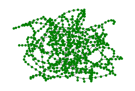
time별 같은 edge 정보를 가지고 있나 확인
np.where(data[0][1].edge_index != data[10][1].edge_index)(array([], dtype=int64), array([], dtype=int64))from torch_geometric_temporal.dataset import MontevideoBusDatasetLoader
loader = MontevideoBusDatasetLoader()
dataset = loader.get_dataset(lags=4)
train_dataset, test_dataset = temporal_signal_split(dataset, train_ratio=0.5)data=[]
for time, snapshot in enumerate(train_dataset):
data.append([time,snapshot])(data[0][1]).x[0], (data[0][1]).y[0](tensor([-0.4200, -0.4200, -0.4200, -0.4200]), tensor(-0.4200))\(t=0\)에서 \(X\)와 \(y\)를 정리하면 아래와 같음.
- X:= \(x_0,x_1,x_2,x_3\)
- y:= \(x_4\)
(data[1][1]).x[0],(data[1][1]).y[0](tensor([-0.4200, -0.4200, -0.4200, -0.4200]), tensor(-0.4200))- X:= \(x_1,x_2,x_3,x_4\)
- y:= \(x_5\)
(data[2][1]).x[0],(data[2][1]).y[0](tensor([-0.4200, -0.4200, -0.4200, -0.4200]), tensor(-0.4200))- X:=\(x_2,x_3,x_4,x_5\)
- y:=\(x_6\)
하나의 노드에 길이가 \(T\)인 시계열이 맵핑되어 있음. (노드는 총 675개)
각 노드마다 아래와 같은 과정으로 예측이 됨
- \((x_0,x_1,x_2,x_3) \to (x_4)\)
- \((x_1,x_2,x_3,x_4) \to (x_5)\)
\(f(v,t), v \in \{v_1,\dots,v_{675}\}, t=1,2,\dots,739\)
\[{\bf X}_{t=1} = \begin{bmatrix} f(v_1,t=1) & f(v_1,t=2) & f(v_1,t=3)& f(v_1,t=4) \\ f(v_2,t=1) & f(v_2,t=2) & f(v_2,t=3)& f(v_2,t=4) \\ \dots & \dots & \dots & \dots \\ f(v_{20},t=1) & f(v_{20},t=2) & f(v_{20},t=3)& f(v_{20},t=4) \end{bmatrix}\]
\[{\bf y}_{t=1} = \begin{bmatrix} f(v_1,t=5) \\ f(v_2,t=5) \\ \dots \\ f(v_{20},t=5) \end{bmatrix}\]
Learn
model = RecurrentGCN(node_features=4, filters=32)

optimizer = torch.optim.Adam(model.parameters(), lr=0.01)

model.train()

for epoch in tqdm(range(50)):
    for time, snapshot in enumerate(train_dataset):
        y_hat = model(snapshot.x, snapshot.edge_index, snapshot.edge_attr)
        cost = torch.mean((y_hat-snapshot.y)**2)
        cost.backward()
        optimizer.step()
optimizer.zero_grad()100%|██████████| 50/50 [01:51<00:00, 2.23s/it]for time, snapshot in enumerate(train_dataset):
_x = snapshot.x
_edge_index = snapshot.edge_index
_edge_attr = snapshot.edge_attr
_y = snapshot.y
break_x.shapetorch.Size([675, 4])_edge_index.shapetorch.Size([2, 690])_edge_attr.shapetorch.Size([690])_y.shapetorch.Size([675])_x.shapetorch.Size([675, 4])x
y
- The target is the passenger inflow.
- This is a curated dataset made from different data sources of the Metropolitan Transportation System (STM) of Montevide
_x[0:3]tensor([[-0.4200, -0.4200, -0.4200, -0.4200],
[-0.0367, -0.0367, -0.0367, -0.0367],
[-0.2655, -0.2655, -0.2655, -0.2655]])_y[:3]tensor([-0.4200, -0.0367, -0.2655])TwitterTennisDatasetLoader
https://appliednetsci.springeropen.com/articles/10.1007/s41109-018-0080-5?ref=https://githubhelp.com
Twitter Tennis RG and UO
- Twitter mention graphs of major tennis tournaments from 2017. Each snapshot contains the graph of popular player or sport news accounts and mentions between them [5, 6]. Node labels encode the number of mentions received and vertex features are structural properties
데이터정리
- T = 52081
- V = 트위터계정
- N = 1000 # number of nodes
- E = 119 = N^2 # edges
- \(f(v,t)\)의 차원? (1,) # passenger inflow
- 시간에 따라서 N이 변하는지? ??
- 시간에 따라서 E가 변하는지? True
- X: ?
- y: ?
- 예제코드적용가능여부: No
- Nodes : 1000
- vertices are Twitter accounts
-Edges : 119
- edges are mentions between them
- Time : 52081
- Twitter mention graphs related to major tennis tournaments from 2017
from torch_geometric_temporal.dataset import TwitterTennisDatasetLoader
from torch_geometric_temporal.signal import temporal_signal_split

loader = TwitterTennisDatasetLoader()

dataset = loader.get_dataset()

train_dataset, test_dataset = temporal_signal_split(dataset, train_ratio=1)data=[]
for time, snapshot in enumerate(train_dataset):
data.append([time,snapshot])time119(data[0][1]).x.shape,(data[0][1]).edge_index.shape,(data[0][1]).edge_attr.shape(torch.Size([1000, 16]), torch.Size([2, 89]), torch.Size([89]))data[0][1].x[0]tensor([0., 0., 0., 0., 1., 1., 0., 0., 0., 0., 0., 0., 0., 0., 0., 0.])data[0][1].edge_index[0]tensor([ 42, 909, 909, 909, 233, 233, 450, 256, 256, 256, 256, 256, 434, 434,
434, 233, 233, 233, 233, 233, 233, 233, 9, 9, 355, 84, 84, 84,
84, 140, 140, 140, 140, 0, 140, 238, 238, 238, 649, 875, 875, 234,
73, 73, 341, 341, 341, 341, 341, 417, 293, 991, 74, 581, 282, 162,
144, 383, 383, 135, 135, 910, 910, 910, 910, 910, 87, 87, 87, 87,
9, 9, 934, 934, 162, 225, 42, 911, 911, 911, 911, 911, 911, 911,
911, 498, 498, 64, 435])data[0][1].edge_attrtensor([2., 1., 1., 1., 1., 1., 1., 1., 1., 1., 1., 1., 1., 1., 1., 1., 1., 1.,
1., 1., 1., 1., 1., 1., 1., 1., 1., 1., 1., 1., 1., 1., 1., 1., 1., 1.,
1., 1., 1., 1., 1., 1., 1., 1., 1., 1., 1., 1., 2., 1., 1., 1., 1., 1.,
1., 1., 1., 1., 1., 1., 1., 1., 1., 1., 2., 2., 1., 1., 1., 1., 1., 1.,
1., 1., 1., 1., 3., 2., 1., 1., 1., 1., 2., 2., 2., 1., 1., 1., 3.])G = nx.Graph()node_list = torch.tensor(range(1000)).tolist()G.add_nodes_from(node_list)edge_list=[]
for i in range(119):
for j in range(40):
edge_list.append([data[i][1].edge_index[0][j].tolist(),data[i][1].edge_index[1][j].tolist()])G.add_edges_from(edge_list)G.number_of_nodes(),G.number_of_edges()(1000, 2819)nx.draw(G,node_color='green',node_size=50,width=1)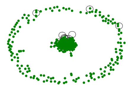
time별 같은 edge 정보를 가지고 있나 확인
len(data[2][1].edge_index[0])67len(data[0][1].edge_index[0])89다름..
from torch_geometric_temporal.dataset import TwitterTennisDatasetLoader
loader = TwitterTennisDatasetLoader()

dataset = loader.get_dataset()

train_dataset, test_dataset = temporal_signal_split(dataset, train_ratio=0.5)data=[]
for time, snapshot in enumerate(train_dataset):
data.append([time,snapshot])(data[0][1]).x[0], (data[0][1]).y[0](tensor([0., 0., 0., 0., 1., 1., 0., 0., 0., 0., 0., 0., 0., 0., 0., 0.]),
tensor(4.8363))(data[1][1]).x[0],(data[1][1]).y[0](tensor([0., 0., 0., 1., 0., 1., 0., 0., 0., 0., 0., 0., 0., 0., 0., 0.]),
tensor(4.9200))(data[2][1]).x[0],(data[2][1]).y[0](tensor([0., 0., 0., 0., 1., 1., 0., 0., 0., 0., 0., 0., 0., 0., 0., 0.]),
tensor(6.5539))(data[3][1]).x[0],(data[3][1]).y[0](tensor([0., 0., 0., 0., 1., 1., 0., 0., 0., 0., 0., 0., 0., 0., 0., 0.]),
tensor(6.9651))for time, snapshot in enumerate(train_dataset):
_x = snapshot.x
_edge_index = snapshot.edge_index
_edge_attr = snapshot.edge_attr
_y = snapshot.y
break_x.shapetorch.Size([1000, 16])_edge_index.shapetorch.Size([2, 89])_edge_attr.shapetorch.Size([89])_y.shapetorch.Size([1000])_x.shapetorch.Size([1000, 16])x
y
_x[0:3]tensor([[0., 0., 0., 0., 1., 1., 0., 0., 0., 0., 0., 0., 0., 0., 0., 0.],
[0., 0., 1., 0., 0., 1., 0., 0., 0., 0., 0., 0., 0., 0., 0., 0.],
[0., 0., 1., 0., 0., 1., 0., 0., 0., 0., 0., 0., 0., 0., 0., 0.]])_y[0]tensor(4.8363)MTMDatasetLoader
MTM-1 Hand Motions
- A temporal dataset of MethodsTime Measurement-1 [36] motions, signalled as consecutive graph frames of 21 3D hand key points that were acquired via MediaPipe Hands [64] from original RGB-Video material. Node features encode the normalized xyz-coordinates of each finger joint and the vertices are connected according to the human hand structure.
데이터정리
- T = 14452
- V = 손의 shape에 대응하는 dot
- N = 325 # number of nodes
- E = 19 = N^2 # edges
- \(f(v,t)\)의 차원? (Grasp, Release, Move, Reach, Poision, -1)
- 시간에 따라서 N이 변하는지? ??
- 시간에 따라서 E가 변하는지? ??
- X: ?
- y: ?
- 예제코드적용가능여부: No
- Nodes : 325
- vertices are are the finger joints of the human hand
-Edges : 19
- edges are the bones connecting them
- Time : 14452
from torch_geometric_temporal.dataset import MTMDatasetLoader
from torch_geometric_temporal.signal import temporal_signal_split

loader = MTMDatasetLoader()

dataset = loader.get_dataset()

train_dataset, test_dataset = temporal_signal_split(dataset, train_ratio=1)data=[]
for time, snapshot in enumerate(train_dataset):
data.append([time,snapshot])time14452(data[0][1]).x.shape,(data[0][1]).edge_index.shape,(data[0][1]).edge_attr.shape(torch.Size([3, 21, 16]), torch.Size([2, 19]), torch.Size([19]))G = nx.Graph()node_list = torch.tensor(range(21)).tolist()G.add_nodes_from(node_list)edge_list=[]
for i in range(14452):
for j in range(len(data[0][1].edge_index[0])):
edge_list.append([data[i][1].edge_index[0][j].tolist(),data[i][1].edge_index[1][j].tolist()])G.add_edges_from(edge_list)G.number_of_nodes(),G.number_of_edges()(21, 19)nx.draw(G,with_labels=True,font_weight='bold',node_color='green',node_size=350,font_color='white',width=1)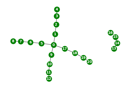
time별 같은 edge 정보를 가지고 있나 확인
np.where(data[0][1].edge_index != data[12][1].edge_index)(array([], dtype=int64), array([], dtype=int64))from torch_geometric_temporal.dataset import MTMDatasetLoader
loader = MTMDatasetLoader()
dataset = loader.get_dataset()
train_dataset, test_dataset = temporal_signal_split(dataset, train_ratio=0.5)data=[]
for time, snapshot in enumerate(train_dataset):
data.append([time,snapshot])(data[0][1]).x[0], (data[0][1]).y[0](tensor([[0., 0., 0., 0., 0., 0., 0., 0., 0., 0., 0., 0., 0., 0., 0., 0.],
[0., 0., 0., 0., 0., 0., 0., 0., 0., 0., 0., 0., 0., 0., 0., 0.],
[0., 0., 0., 0., 0., 0., 0., 0., 0., 0., 0., 0., 0., 0., 0., 0.],
[0., 0., 0., 0., 0., 0., 0., 0., 0., 0., 0., 0., 0., 0., 0., 0.],
[0., 0., 0., 0., 0., 0., 0., 0., 0., 0., 0., 0., 0., 0., 0., 0.],
[0., 0., 0., 0., 0., 0., 0., 0., 0., 0., 0., 0., 0., 0., 0., 0.],
[0., 0., 0., 0., 0., 0., 0., 0., 0., 0., 0., 0., 0., 0., 0., 0.],
[0., 0., 0., 0., 0., 0., 0., 0., 0., 0., 0., 0., 0., 0., 0., 0.],
[0., 0., 0., 0., 0., 0., 0., 0., 0., 0., 0., 0., 0., 0., 0., 0.],
[0., 0., 0., 0., 0., 0., 0., 0., 0., 0., 0., 0., 0., 0., 0., 0.],
[0., 0., 0., 0., 0., 0., 0., 0., 0., 0., 0., 0., 0., 0., 0., 0.],
[0., 0., 0., 0., 0., 0., 0., 0., 0., 0., 0., 0., 0., 0., 0., 0.],
[0., 0., 0., 0., 0., 0., 0., 0., 0., 0., 0., 0., 0., 0., 0., 0.],
[0., 0., 0., 0., 0., 0., 0., 0., 0., 0., 0., 0., 0., 0., 0., 0.],
[0., 0., 0., 0., 0., 0., 0., 0., 0., 0., 0., 0., 0., 0., 0., 0.],
[0., 0., 0., 0., 0., 0., 0., 0., 0., 0., 0., 0., 0., 0., 0., 0.],
[0., 0., 0., 0., 0., 0., 0., 0., 0., 0., 0., 0., 0., 0., 0., 0.],
[0., 0., 0., 0., 0., 0., 0., 0., 0., 0., 0., 0., 0., 0., 0., 0.],
[0., 0., 0., 0., 0., 0., 0., 0., 0., 0., 0., 0., 0., 0., 0., 0.],
[0., 0., 0., 0., 0., 0., 0., 0., 0., 0., 0., 0., 0., 0., 0., 0.],
[0., 0., 0., 0., 0., 0., 0., 0., 0., 0., 0., 0., 0., 0., 0., 0.]]),
tensor([0., 0., 1., 0., 0., 0.]))(data[1][1]).x[0],(data[1][1]).y[0](tensor([[0., 0., 0., 0., 0., 0., 0., 0., 0., 0., 0., 0., 0., 0., 0., 0.],
[0., 0., 0., 0., 0., 0., 0., 0., 0., 0., 0., 0., 0., 0., 0., 0.],
[0., 0., 0., 0., 0., 0., 0., 0., 0., 0., 0., 0., 0., 0., 0., 0.],
[0., 0., 0., 0., 0., 0., 0., 0., 0., 0., 0., 0., 0., 0., 0., 0.],
[0., 0., 0., 0., 0., 0., 0., 0., 0., 0., 0., 0., 0., 0., 0., 0.],
[0., 0., 0., 0., 0., 0., 0., 0., 0., 0., 0., 0., 0., 0., 0., 0.],
[0., 0., 0., 0., 0., 0., 0., 0., 0., 0., 0., 0., 0., 0., 0., 0.],
[0., 0., 0., 0., 0., 0., 0., 0., 0., 0., 0., 0., 0., 0., 0., 0.],
[0., 0., 0., 0., 0., 0., 0., 0., 0., 0., 0., 0., 0., 0., 0., 0.],
[0., 0., 0., 0., 0., 0., 0., 0., 0., 0., 0., 0., 0., 0., 0., 0.],
[0., 0., 0., 0., 0., 0., 0., 0., 0., 0., 0., 0., 0., 0., 0., 0.],
[0., 0., 0., 0., 0., 0., 0., 0., 0., 0., 0., 0., 0., 0., 0., 0.],
[0., 0., 0., 0., 0., 0., 0., 0., 0., 0., 0., 0., 0., 0., 0., 0.],
[0., 0., 0., 0., 0., 0., 0., 0., 0., 0., 0., 0., 0., 0., 0., 0.],
[0., 0., 0., 0., 0., 0., 0., 0., 0., 0., 0., 0., 0., 0., 0., 0.],
[0., 0., 0., 0., 0., 0., 0., 0., 0., 0., 0., 0., 0., 0., 0., 0.],
[0., 0., 0., 0., 0., 0., 0., 0., 0., 0., 0., 0., 0., 0., 0., 0.],
[0., 0., 0., 0., 0., 0., 0., 0., 0., 0., 0., 0., 0., 0., 0., 0.],
[0., 0., 0., 0., 0., 0., 0., 0., 0., 0., 0., 0., 0., 0., 0., 0.],
[0., 0., 0., 0., 0., 0., 0., 0., 0., 0., 0., 0., 0., 0., 0., 0.],
[0., 0., 0., 0., 0., 0., 0., 0., 0., 0., 0., 0., 0., 0., 0., 0.]]),
tensor([0., 0., 1., 0., 0., 0.]))for time, snapshot in enumerate(train_dataset):
_x = snapshot.x
_edge_index = snapshot.edge_index
_edge_attr = snapshot.edge_attr
_y = snapshot.y
break_x.shapetorch.Size([3, 21, 16])_edge_index.shapetorch.Size([2, 19])_edge_attr.shapetorch.Size([19])_y.shapetorch.Size([16, 6])_x.shapetorch.Size([3, 21, 16])x
- The data x is returned in shape (3, 21, T),
y
- The targets are manually labeled for each frame, according to one of the five MTM-1 motions (classes ): Grasp, Release, Move, Reach, Position plus a negative class for frames without graph signals (no hand present).
- the target is returned one-hot-encoded in shape (T, 6).
_x[0]tensor([[0., 0., 0., 0., 0., 0., 0., 0., 0., 0., 0., 0., 0., 0., 0., 0.],
[0., 0., 0., 0., 0., 0., 0., 0., 0., 0., 0., 0., 0., 0., 0., 0.],
[0., 0., 0., 0., 0., 0., 0., 0., 0., 0., 0., 0., 0., 0., 0., 0.],
[0., 0., 0., 0., 0., 0., 0., 0., 0., 0., 0., 0., 0., 0., 0., 0.],
[0., 0., 0., 0., 0., 0., 0., 0., 0., 0., 0., 0., 0., 0., 0., 0.],
[0., 0., 0., 0., 0., 0., 0., 0., 0., 0., 0., 0., 0., 0., 0., 0.],
[0., 0., 0., 0., 0., 0., 0., 0., 0., 0., 0., 0., 0., 0., 0., 0.],
[0., 0., 0., 0., 0., 0., 0., 0., 0., 0., 0., 0., 0., 0., 0., 0.],
[0., 0., 0., 0., 0., 0., 0., 0., 0., 0., 0., 0., 0., 0., 0., 0.],
[0., 0., 0., 0., 0., 0., 0., 0., 0., 0., 0., 0., 0., 0., 0., 0.],
[0., 0., 0., 0., 0., 0., 0., 0., 0., 0., 0., 0., 0., 0., 0., 0.],
[0., 0., 0., 0., 0., 0., 0., 0., 0., 0., 0., 0., 0., 0., 0., 0.],
[0., 0., 0., 0., 0., 0., 0., 0., 0., 0., 0., 0., 0., 0., 0., 0.],
[0., 0., 0., 0., 0., 0., 0., 0., 0., 0., 0., 0., 0., 0., 0., 0.],
[0., 0., 0., 0., 0., 0., 0., 0., 0., 0., 0., 0., 0., 0., 0., 0.],
[0., 0., 0., 0., 0., 0., 0., 0., 0., 0., 0., 0., 0., 0., 0., 0.],
[0., 0., 0., 0., 0., 0., 0., 0., 0., 0., 0., 0., 0., 0., 0., 0.],
[0., 0., 0., 0., 0., 0., 0., 0., 0., 0., 0., 0., 0., 0., 0., 0.],
[0., 0., 0., 0., 0., 0., 0., 0., 0., 0., 0., 0., 0., 0., 0., 0.],
[0., 0., 0., 0., 0., 0., 0., 0., 0., 0., 0., 0., 0., 0., 0., 0.],
[0., 0., 0., 0., 0., 0., 0., 0., 0., 0., 0., 0., 0., 0., 0., 0.]])_y[0]tensor([0., 0., 1., 0., 0., 0.])