DNN (4주차)

기계학습 특강 (4주차) 9월28일 [회귀분석(2)–step1~4, step1의 다른표현, step4의 다른표현, 로지스틱 intro]

imports

import numpy as np
import matplotlib.pyplot as plt 
import pandas as pd
import torch

numpy, torch (선택학습)

numpy, torch는 엄청 비슷해요

- torch.tensor() = np.array() 처럼 생각해도 무방

np.array([1,2,3]), torch.tensor([1,2,3])

(array([1, 2, 3]), tensor([1, 2, 3]))

- 소수점의 정밀도에서 차이가 있음 (torch가 좀 더 쪼잔함)

np.array([3.123456789])

array([3.12345679])

torch.tensor([3.123456789])

tensor([3.1235])

(서연필기)tensor는 gpu에 저장하기 때문에 메모리 아끼기 위해 정밀도가 낮은 경향이 있다.

- 기본적인 numpy 문법은 np 대신에 torch를 써도 무방 // 완전 같지는 않음

np.arange(10), torch.arange(10)

(array([0, 1, 2, 3, 4, 5, 6, 7, 8, 9]), tensor([0, 1, 2, 3, 4, 5, 6, 7, 8, 9]))

np.linspace(0,1,10), torch.linspace(0,1,10)

(array([0.        , 0.11111111, 0.22222222, 0.33333333, 0.44444444,
        0.55555556, 0.66666667, 0.77777778, 0.88888889, 1.        ]),
 tensor([0.0000, 0.1111, 0.2222, 0.3333, 0.4444, 0.5556, 0.6667, 0.7778, 0.8889,
         1.0000]))

np.random.randn(10)

array([-0.90388568,  0.51779102,  0.73699131, -0.88030899,  1.71668715,
       -0.70735651, -0.29752154,  1.10432159,  0.23592126,  0.91669421])

torch.randn(10)

tensor([ 0.6896,  1.8534, -0.3807,  1.3676,  0.0515,  0.4350,  0.6051, -1.5075,
         0.1474,  0.3098])

length \(n\) vector, \(n \times 1\) col-vector, \(1 \times n\) row-vector

브로드캐스팅 길이가 3인 벡터와 1인벡터를 더하면 오류 뜨지 않고 더해줌

- 길이가 3인 벡터 선언방법

a = torch.tensor([1,2,3])
a.shape

torch.Size([3])

- 3x1 col-vec 선언방법

(방법1)

a = torch.tensor([[1],[2],[3]])
a.shape

torch.Size([3, 1])

(방법2)

a = torch.tensor([1,2,3]).reshape(3,1)
a.shape

torch.Size([3, 1])

- 1x3 row-vec 선언방법

(방법1)

a = torch.tensor([[1,2,3]])
a.shape

torch.Size([1, 3])

(방법2)

a = torch.tensor([1,2,3]).reshape(1,3)
a.shape

torch.Size([1, 3])

- 3x1 col-vec 선언방법, 1x3 row-vec 선언방법에서 [[1],[2],[3]] 혹은 [[1,2,3]] 와 같은 표현이 이해안되면 아래링크로 가셔서

https://guebin.github.io/STBDA2022/2022/03/14/(2주차)-3월14일.html

첫번째 동영상 12:15 - 22:45 에 해당하는 분량을 학습하시길 바랍니다.

torch의 dtype

- 기본적으로 torch는 소수점으로 저장되면 dtype=torch.float32 가 된다. (이걸로 맞추는게 편리함)

tsr = torch.tensor([1.23,2.34])
tsr

tensor([1.2300, 2.3400])

tsr.dtype

torch.float32

- 정수로 선언하더라도 dtype를 torch.float32로 바꾸는게 유리함

(안 좋은 선언예시)

tsr = torch.tensor([1,2])
tsr 

tensor([1, 2])

tsr.dtype

torch.int64

(좋은 선언예시1)

tsr = torch.tensor([1,2],dtype=torch.float32)
tsr 

tensor([1., 2.])

tsr.dtype

torch.float32

(좋은 선언예시2)

tsr = torch.tensor([1,2.0])
tsr 

tensor([1., 2.])

tsr.dtype

torch.float32

(사실 int로 선언해도 나중에 float으로 바꾸면 큰 문제없음)

tsr = torch.tensor([1,2]).float()
tsr

tensor([1., 2.])

tsr.dtype

torch.float32

- 왜 정수만으로 torch.tensor를 만들때에도 torch.float32로 바꾸는게 유리할까? \(\to\) torch.tensor끼리의 연산에서 문제가 될 수 있음

별 문제 없을수도 있지만

torch.tensor([1,2])-torch.tensor([1.0,2.0]) 

tensor([0., 0.])

아래와 같이 에러가 날수도 있다

(에러1)

torch.tensor([[1.0,0.0],[0.0,1.0]]) @ torch.tensor([[1],[2]]) 

RuntimeError: expected scalar type Float but found Long

(에러2)

torch.tensor([[1,0],[0,1]]) @ torch.tensor([[1.0],[2.0]])

RuntimeError: expected scalar type Long but found Float

(해결1) 둘다 정수로 통일

torch.tensor([[1,0],[0,1]]) @ torch.tensor([[1],[2]])

tensor([[1],
        [2]])

(해결2) 둘다 소수로 통일 <– 더 좋은 방법임

torch.tensor([[1.0,0.0],[0.0,1.0]]) @ torch.tensor([[1.0],[2.0]])

tensor([[1.],
        [2.]])

shape of vector

- 행렬곱셈에 대한 shape 조심

A = torch.tensor([[2.00,0.00],[0.00,3.00]]) 
b1 = torch.tensor([[-1.0,-5.0]])
b2 = torch.tensor([[-1.0],[-5.0]])
b3 = torch.tensor([-1.0,-5.0])

A.shape,b1.shape,b2.shape,b3.shape

(torch.Size([2, 2]), torch.Size([1, 2]), torch.Size([2, 1]), torch.Size([2]))

- A@b1: 계산불가, b1@A: 계산가능

A@b1

RuntimeError: mat1 and mat2 shapes cannot be multiplied (2x2 and 1x2)

b1@A

tensor([[ -2., -15.]])

- A@b2: 계산가능, b2@A: 계산불가

A@b2

tensor([[ -2.],
        [-15.]])

b2@A

RuntimeError: mat1 and mat2 shapes cannot be multiplied (2x1 and 2x2)

- A@b3: 계산가능, b3@A: 계산가능

(A@b3).shape ## b3를 마치 col-vec 처럼 해석

torch.Size([2])

(b3@A).shape ## b3를 마지 row-vec 처럼 해석

torch.Size([2])

• 뒤에 놓으면 b3를 컬럼벡터로 인식
• 앞에 놓으면 b3를 로우벡터로 인식

- 브로드캐스팅

a = torch.tensor([1,2,3])
a - 1

tensor([0, 1, 2])

b = torch.tensor([[1],[2],[3]])
b - 1

tensor([[0],
        [1],
        [2]])

계산이 되지 않아야 맞지 않나

a - b # a를 row-vec 로 해석

tensor([[ 0,  1,  2],
        [-1,  0,  1],
        [-2, -1,  0]])

잘못 계싼할 수 있으니 dimension 명시해주자

Review: step1~4

df = pd.read_csv("https://raw.githubusercontent.com/guebin/DL2022/master/_notebooks/2022-09-22-regression.csv") 
df

	x	y
0	-2.482113	-8.542024
1	-2.362146	-6.576713
2	-1.997295	-5.949576
3	-1.623936	-4.479364
4	-1.479192	-4.251570
...	...	...
95	2.244400	10.325987
96	2.393501	12.266493
97	2.605604	13.098280
98	2.605658	12.546793
99	2.663240	13.834002

100 rows × 2 columns

plt.plot(df.x, df.y,'o')

torch.tensor(df.x)

tensor([-2.4821, -2.3621, -1.9973, -1.6239, -1.4792, -1.4635, -1.4509, -1.4435,
        -1.3722, -1.3079, -1.1904, -1.1092, -1.1054, -1.0875, -0.9469, -0.9319,
        -0.8643, -0.7858, -0.7549, -0.7421, -0.6948, -0.6103, -0.5830, -0.5621,
        -0.5506, -0.5058, -0.4806, -0.4738, -0.4710, -0.4676, -0.3874, -0.3719,
        -0.3688, -0.3159, -0.2775, -0.2772, -0.2734, -0.2721, -0.2668, -0.2155,
        -0.2000, -0.1816, -0.1708, -0.1565, -0.1448, -0.1361, -0.1057, -0.0603,
        -0.0559, -0.0214,  0.0655,  0.0684,  0.1195,  0.1420,  0.1521,  0.1568,
         0.2646,  0.2656,  0.3157,  0.3220,  0.3461,  0.3984,  0.4190,  0.5443,
         0.5579,  0.5913,  0.6148,  0.6469,  0.6469,  0.6523,  0.6674,  0.7059,
         0.7141,  0.7822,  0.8154,  0.8668,  0.9291,  0.9804,  0.9853,  0.9941,
         1.0376,  1.0393,  1.0697,  1.1024,  1.1126,  1.1532,  1.2289,  1.3403,
         1.3494,  1.4279,  1.4994,  1.5031,  1.5437,  1.6789,  2.0832,  2.2444,
         2.3935,  2.6056,  2.6057,  2.6632], dtype=torch.float64)

(서연필기)

float64 숫자 정밀 저장

float32이면 dtype=torch.float64)꼬리표가 붙지 않음

_trt = torch.tensor(df.x).float()
_trt = torch.tensor(df.x,dtype=float30)

같은 역할, 메모리 적게 쓰기 위해 타입 바꿔주자

x= torch.tensor(df.x,dtype=torch.float32).reshape(100,1)

컬럼형식으로 받아주기 위해 변경

x= torch.tensor(df.x,dtype=torch.float32).reshape(100,1)
y= torch.tensor(df.y,dtype=torch.float32).reshape(100,1)
_1= torch.ones([100,1])
X = torch.concat([_1,x],axis=1)

torch.ones([100,1])
torch.tensor([[1]*100,x]).T

같은 셋

What = torch.tensor([[-5.0],[10.0]],requires_grad=True)
What

tensor([[-5.],
        [10.]], requires_grad=True)

requires_grad=True 

reshape 미분 가능 옵션 주기 전에 shape 정해주자

plt.plot(x,y,'o')
#plt.plot(x,-5+10*x,'--')
plt.plot(x,X@What.data,'--')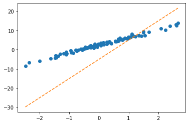

ver1: loss = sum of squares error

alpha = 1/1000
What = torch.tensor([[-5.0],[10.0]],requires_grad=True)
for epoc in range(30): 
    # step1: yhat 
    yhat = X@What 
    # step2: loss 
    loss = torch.sum((y-yhat)**2)
    # step3: 미분 
    loss.backward()
    # step4: update 
    What.data = What.data - alpha * What.grad 
    What.grad = None # 

What

tensor([[2.4290],
        [4.0144]], requires_grad=True)

plt.plot(x,y,'o') 
plt.plot(x,X@What.data,'--')

• note: 왜 What = What - alpha*What.grad 는 안되는지?

What

tensor([[2.4290],
        [4.0144]], requires_grad=True)

What.data

tensor([[2.4290],
        [4.0144]])

What과 What.data는 달라요, requires_grad=True 미분 가능 꼬리표가 붙지 않기 때문!

ver2: loss = mean squared error = MSE

alpha = 1/10
What = torch.tensor([[-5.0],[10.0]],requires_grad=True)
for epoc in range(30): 
    # step1: yhat 
    yhat = X@What 
    # step2: loss 
    loss = torch.mean((y-yhat)**2)
    # step3: 미분 
    loss.backward()
    # step4: update 
    What.data = What.data - alpha * What.grad 
    What.grad = None # 

What

tensor([[2.4290],
        [4.0144]], requires_grad=True)

(서연필기)mean 정의 - 데이터를 더 효율적으로 학습 가능, 데이터 수만큼 안 해도 돼, 계산 덜 해도 돼

step1의 다른버전 – net 설계만

ver1: net = torch.nn.Linear(1,1,bias=True)

torch.nn.Linear?

Init signature:
torch.nn.Linear(
    in_features: int,
    out_features: int,
    bias: bool = True,
    device=None,
    dtype=None,
) -> None
Docstring:     
Applies a linear transformation to the incoming data: :math:`y = xA^T + b`
This module supports :ref:`TensorFloat32<tf32_on_ampere>`.
Args:
    in_features: size of each input sample
    out_features: size of each output sample
    bias: If set to ``False``, the layer will not learn an additive bias.
        Default: ``True``
Shape:
    - Input: :math:`(*, H_{in})` where :math:`*` means any number of
      dimensions including none and :math:`H_{in} = \text{in\_features}`.
    - Output: :math:`(*, H_{out})` where all but the last dimension
      are the same shape as the input and :math:`H_{out} = \text{out\_features}`.
Attributes:
    weight: the learnable weights of the module of shape
        :math:`(\text{out\_features}, \text{in\_features})`. The values are
        initialized from :math:`\mathcal{U}(-\sqrt{k}, \sqrt{k})`, where
        :math:`k = \frac{1}{\text{in\_features}}`
    bias:   the learnable bias of the module of shape :math:`(\text{out\_features})`.
            If :attr:`bias` is ``True``, the values are initialized from
            :math:`\mathcal{U}(-\sqrt{k}, \sqrt{k})` where
            :math:`k = \frac{1}{\text{in\_features}}`
Examples::
    >>> m = nn.Linear(20, 30)
    >>> input = torch.randn(128, 20)
    >>> output = m(input)
    >>> print(output.size())
    torch.Size([128, 30])
Init docstring: Initializes internal Module state, shared by both nn.Module and ScriptModule.
File:           ~/anaconda3/envs/csy/lib/python3.8/site-packages/torch/nn/modules/linear.py
Type:           type
Subclasses:     NonDynamicallyQuantizableLinear, LazyLinear, Linear, Linear

input 잡는 법 - x의 컬럼 부분을 input이라고 생각하자

x.shape

torch.Size([100, 1])

output 잡는 법 - y의 컬럼 부분을 output이라고 생각하자

y.shape

torch.Size([100, 1])

_net =  torch.nn.Linear(in_features=1, out_features=1, bias=True) 

_net(x).shape

torch.Size([100, 1])

_net.bias # w0

Parameter containing:
tensor([-0.1281], requires_grad=True)

_net.weight # w1

Parameter containing:
tensor([[0.1433]], requires_grad=True)

torch.manual_seed(43052)
net = torch.nn.Linear(in_features=1, out_features=1, bias=True) 

net.bias, net.weight

(Parameter containing:
 tensor([-0.8470], requires_grad=True),
 Parameter containing:
 tensor([[-0.3467]], requires_grad=True))

plt.plot(x,y,'o')
plt.plot(x,net(x).data,'--')
w0hat = -0.847
w1hat = -0.3467
plt.plot(x,w0hat+w1hat*x,'--')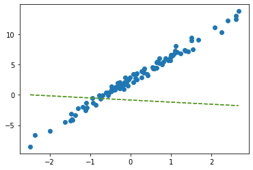

출력결과 같음을 확인

- net에서 \(\hat{w}_0, \hat{w}_1\) 의 값은?

net.weight # w1 

Parameter containing:
tensor([[-0.3467]], requires_grad=True)

net.bias # w0 

Parameter containing:
tensor([-0.8470], requires_grad=True)

_yhat = -0.8470 + -0.3467*x 

plt.plot(x,y,'o')
plt.plot(x, _yhat,'--')
plt.plot(x,net(x).data,'-.')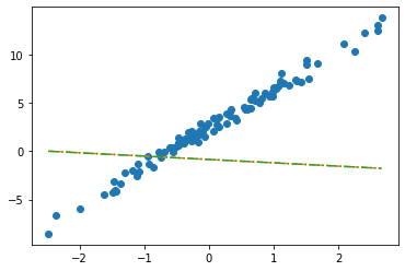

- 수식표현: \(\hat{y}_i = \hat{w}_0 + \hat{w}_1 x_i = \hat{b} + \hat{w}x_i = -0.8470 + -0.3467 x_i\) for all \(i=1,2,\dots,100\).

ver2: net = torch.nn.Linear(2,1,bias=False)

- 입력이 x가 아닌 X를 넣고 싶다면? (보통 잘 안하긴 해요, 왜? bias=False로 주는게 귀찮거든요) - X는 바이어스가 고려된 상황

net(X) ## 그대로 쓰면 당연히 에러

RuntimeError: mat1 and mat2 shapes cannot be multiplied (100x2 and 1x1)

torch.manual_seed(43052)
net = torch.nn.Linear(in_features=2, out_features=1, bias=False) 

net(X).shape

torch.Size([100, 1])

net.weight

Parameter containing:
tensor([[-0.2451, -0.5989]], requires_grad=True)

위에 \(w_0,w_1\) 순

net.bias

bias 없음을 확인

plt.plot(x,y,'o') 
plt.plot(x,net(X).data, '--')
plt.plot(x,X@torch.tensor([[-0.2451],[-0.5989]]), '-.')

- 수식표현: \(\hat{\bf y} = {\bf X} {\bf \hat W} = \begin{bmatrix} 1 & x_1 \\ 1 & x_2 \\ \dots & \dots \\ 1 & x_{100} \end{bmatrix} \begin{bmatrix} -0.2451 \\ -0.5989 \end{bmatrix}\)

잘못된사용1

_x = x.reshape(-1)

_x

tensor([-2.4821, -2.3621, -1.9973, -1.6239, -1.4792, -1.4635, -1.4509, -1.4435,
        -1.3722, -1.3079, -1.1904, -1.1092, -1.1054, -1.0875, -0.9469, -0.9319,
        -0.8643, -0.7858, -0.7549, -0.7421, -0.6948, -0.6103, -0.5830, -0.5621,
        -0.5506, -0.5058, -0.4806, -0.4738, -0.4710, -0.4676, -0.3874, -0.3719,
        -0.3688, -0.3159, -0.2775, -0.2772, -0.2734, -0.2721, -0.2668, -0.2155,
        -0.2000, -0.1816, -0.1708, -0.1565, -0.1448, -0.1361, -0.1057, -0.0603,
        -0.0559, -0.0214,  0.0655,  0.0684,  0.1195,  0.1420,  0.1521,  0.1568,
         0.2646,  0.2656,  0.3157,  0.3220,  0.3461,  0.3984,  0.4190,  0.5443,
         0.5579,  0.5913,  0.6148,  0.6469,  0.6469,  0.6523,  0.6674,  0.7059,
         0.7141,  0.7822,  0.8154,  0.8668,  0.9291,  0.9804,  0.9853,  0.9941,
         1.0376,  1.0393,  1.0697,  1.1024,  1.1126,  1.1532,  1.2289,  1.3403,
         1.3494,  1.4279,  1.4994,  1.5031,  1.5437,  1.6789,  2.0832,  2.2444,
         2.3935,  2.6056,  2.6057,  2.6632])

torch.manual_seed(43052)
net = torch.nn.Linear(in_features=1,out_features=1) 

net(_x)

RuntimeError: mat1 and mat2 shapes cannot be multiplied (1x100 and 1x1)

net(_x.reshape(100,1))

과 같이 정의

잘못된사용2

torch.manual_seed(43052)
net = torch.nn.Linear(in_features=2,out_features=1) # bias=False를 깜빡..

net.weight

Parameter containing:
tensor([[-0.2451, -0.5989]], requires_grad=True)

net.bias

Parameter containing:
tensor([0.2549], requires_grad=True)

plt.plot(x,y,'o')
plt.plot(x,net(X).data,'--')
plt.plot(x,X@torch.tensor([[-0.2451],[-0.5989]])+0.2549,'-.')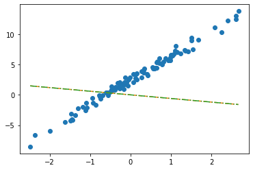

• 수식표현: \(\hat{\bf y} = {\bf X} {\bf \hat W} + \hat{b}= \begin{bmatrix} 1 & x_1 \\ 1 & x_2 \\ \dots & \dots \\ 1 & x_{100} \end{bmatrix} \begin{bmatrix} -0.2451 \\ -0.5989 \end{bmatrix} + 0.2549\)

step1의 다른버전 – 끝까지

ver1: net = torch.nn.Linear(1,1,bias=True)

- 준비

net = torch.nn.Linear(1,1,bias=True)
net.weight.data = torch.tensor([[10.0]])
net.bias.data = torch.tensor([-5.0])
net.weight,net.bias

(Parameter containing:
 tensor([[10.]], requires_grad=True),
 Parameter containing:
 tensor([-5.], requires_grad=True))

- step1

yhat = net(x) 

plt.plot(x,y,'o')
plt.plot(x,net(x).data,'--')
plt.plot(x,-5+10*x,'--')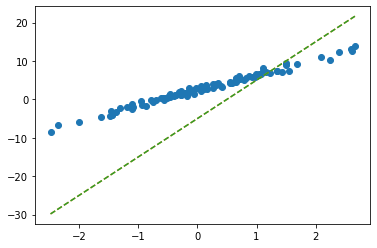

- step2

loss = torch.mean((y-yhat)**2)

- step3

(미분전)

net.bias,net.weight

(Parameter containing:
 tensor([-5.], requires_grad=True),
 Parameter containing:
 tensor([[10.]], requires_grad=True))

net.bias.grad, net.weight.grad

(None, None)

(미분)

loss.backward()

(미분후)

net.bias,net.weight

(Parameter containing:
 tensor([-5.], requires_grad=True),
 Parameter containing:
 tensor([[10.]], requires_grad=True))

net.bias.grad,net.weight.grad

(tensor([-13.4225]), tensor([[11.8893]]))

- step4

(업데이트전)

net.bias,net.weight

(Parameter containing:
 tensor([-5.], requires_grad=True),
 Parameter containing:
 tensor([[10.]], requires_grad=True))

net.bias.grad, net.weight.grad

(tensor([-13.4225]), tensor([[11.8893]]))

(업데이트)

net.bias.data = net.bias.data - 0.1*net.bias.grad 
net.weight.data = net.weight.data - 0.1*net.weight.grad 

net.bias.grad = None 
net.weight.grad = None 

(업데이트후)

net.bias,net.weight

(Parameter containing:
 tensor([-3.6577], requires_grad=True),
 Parameter containing:
 tensor([[8.8111]], requires_grad=True))

net.bias.grad, net.weight.grad

(None, None)

- 반복

net = torch.nn.Linear(1,1)
net.weight.data = torch.tensor([[10.0]])
net.bias.data = torch.tensor([-5.0])

for epoc in range(30):
    yhat = net(x) 
    loss = torch.mean((y-yhat)**2)
    loss.backward()
    net.weight.data = net.weight.data - 0.1*net.weight.grad
    net.bias.data = net.bias.data - 0.1*net.bias.grad
    net.weight.grad = None
    net.bias.grad = None

plt.plot(x,y,'o')
plt.plot(x,net(x).data,'--')

ver2: net = torch.nn.Linear(2,1,bias=False)

- 준비

net = torch.nn.Linear(2,1,bias=False)
net.weight.data = torch.tensor([[-5.0, 10.0]])

- step1

yhat = net(X)

- step2

loss = torch.mean((y-yhat)**2)

- step3

(미분전)

net.weight

Parameter containing:
tensor([[-5., 10.]], requires_grad=True)

net.weight.grad

(미분)

loss.backward()

(미분후)

net.weight

Parameter containing:
tensor([[-5., 10.]], requires_grad=True)

net.weight.grad

tensor([[-13.4225,  11.8893]])

- step4

(업데이트전)

net.weight

Parameter containing:
tensor([[-5., 10.]], requires_grad=True)

net.weight.grad

tensor([[-13.4225,  11.8893]])

(업데이트)

net.weight.data = net.weight.data - 0.1*net.weight.grad

net.weight.grad = None

(업데이트후)

net.weight

Parameter containing:
tensor([[-3.6577,  8.8111]], requires_grad=True)

net.weight.grad

- 반복

net = torch.nn.Linear(2,1,bias=False)
net.weight.data = torch.tensor([[-5.0, 10.0]])

plt.plot(x,y,'o')
plt.plot(x,net(X).data,'--')

for epoc in range(30):
    yhat = net(X) 
    loss = torch.mean((y-yhat)**2)
    loss.backward()
    net.weight.data = net.weight.data - 0.1*net.weight.grad
    net.weight.grad = None

plt.plot(x,y,'o')
plt.plot(x,net(X).data,'--')

step4의 다른버전: 옵티마이저!

ver1: net = torch.nn.Linear(1,1,bias=True)

- 준비

net = torch.nn.Linear(1,1) 
net.weight.data = torch.tensor([[10.0]]) 
net.bias.data = torch.tensor([[-5.0]]) 

torch.optim.SGD?

Init signature:
torch.optim.SGD(
    params,
    lr=<required parameter>,
    momentum=0,
    dampening=0,
    weight_decay=0,
    nesterov=False,
)
Docstring:     
Implements stochastic gradient descent (optionally with momentum).
.. math::
   \begin{aligned}
        &\rule{110mm}{0.4pt}                                                                 \\
        &\textbf{input}      : \gamma \text{ (lr)}, \: \theta_0 \text{ (params)}, \: f(\theta)
            \text{ (objective)}, \: \lambda \text{ (weight decay)},                          \\
        &\hspace{13mm} \:\mu \text{ (momentum)}, \:\tau \text{ (dampening)},\:nesterov\\[-1.ex]
        &\rule{110mm}{0.4pt}                                                                 \\
        &\textbf{for} \: t=1 \: \textbf{to} \: \ldots \: \textbf{do}                         \\
        &\hspace{5mm}g_t           \leftarrow   \nabla_{\theta} f_t (\theta_{t-1})           \\
        &\hspace{5mm}\textbf{if} \: \lambda \neq 0                                           \\
        &\hspace{10mm} g_t \leftarrow g_t + \lambda  \theta_{t-1}                            \\
        &\hspace{5mm}\textbf{if} \: \mu \neq 0                                               \\
        &\hspace{10mm}\textbf{if} \: t > 1                                                   \\
        &\hspace{15mm} \textbf{b}_t \leftarrow \mu \textbf{b}_{t-1} + (1-\tau) g_t           \\
        &\hspace{10mm}\textbf{else}                                                          \\
        &\hspace{15mm} \textbf{b}_t \leftarrow g_t                                           \\
        &\hspace{10mm}\textbf{if} \: nesterov                                                \\
        &\hspace{15mm} g_t \leftarrow g_{t-1} + \mu \textbf{b}_t                             \\
        &\hspace{10mm}\textbf{else}                                                   \\[-1.ex]
        &\hspace{15mm} g_t  \leftarrow  \textbf{b}_t                                         \\
        &\hspace{5mm}\theta_t \leftarrow \theta_{t-1} - \gamma g_t                    \\[-1.ex]
        &\rule{110mm}{0.4pt}                                                          \\[-1.ex]
        &\bf{return} \:  \theta_t                                                     \\[-1.ex]
        &\rule{110mm}{0.4pt}                                                          \\[-1.ex]
   \end{aligned}
Nesterov momentum is based on the formula from
`On the importance of initialization and momentum in deep learning`__.
Args:
    params (iterable): iterable of parameters to optimize or dicts defining
        parameter groups
    lr (float): learning rate
    momentum (float, optional): momentum factor (default: 0)
    weight_decay (float, optional): weight decay (L2 penalty) (default: 0)
    dampening (float, optional): dampening for momentum (default: 0)
    nesterov (bool, optional): enables Nesterov momentum (default: False)
Example:
    >>> optimizer = torch.optim.SGD(model.parameters(), lr=0.1, momentum=0.9)
    >>> optimizer.zero_grad()
    >>> loss_fn(model(input), target).backward()
    >>> optimizer.step()
__ http://www.cs.toronto.edu/%7Ehinton/absps/momentum.pdf
.. note::
    The implementation of SGD with Momentum/Nesterov subtly differs from
    Sutskever et. al. and implementations in some other frameworks.
    Considering the specific case of Momentum, the update can be written as
    .. math::
        \begin{aligned}
            v_{t+1} & = \mu * v_{t} + g_{t+1}, \\
            p_{t+1} & = p_{t} - \text{lr} * v_{t+1},
        \end{aligned}
    where :math:`p`, :math:`g`, :math:`v` and :math:`\mu` denote the
    parameters, gradient, velocity, and momentum respectively.
    This is in contrast to Sutskever et. al. and
    other frameworks which employ an update of the form
    .. math::
        \begin{aligned}
            v_{t+1} & = \mu * v_{t} + \text{lr} * g_{t+1}, \\
            p_{t+1} & = p_{t} - v_{t+1}.
        \end{aligned}
    The Nesterov version is analogously modified.
File:           ~/anaconda3/envs/csy/lib/python3.8/site-packages/torch/optim/sgd.py
Type:           type
Subclasses:     

Stocastic Gradiant Decscent

net.parameters()

<generator object Module.parameters at 0x7f5f0d522740>

optimizr = torch.optim.SGD(net.parameters(),lr=1/10) 

- step1~3

yhat = net(x)     

loss = torch.mean((y-yhat)**2) 

loss.backward() 

- step4

(update 전)

net.weight.data, net.bias.data ## 값은 업데이트 전

(tensor([[10.]]), tensor([[-5.]]))

net.weight.grad, net.bias.grad ## 미분값은 청소전 

(tensor([[11.8893]]), tensor([[-13.4225]]))

(update)

optimizr.step() 
optimizr.zero_grad() 

(update 후)

net.weight.data, net.bias.data ## 값은 업데이트 되었음 

(tensor([[8.8111]]), tensor([[-3.6577]]))

net.weight.grad, net.bias.grad ## 미분값은 0으로 초기화하였음 

(tensor([[0.]]), tensor([[0.]]))

- 반복

net = torch.nn.Linear(1,1) 
net.weight.data = torch.tensor([[10.0]])
net.bias.data = torch.tensor([-5.0])
optimizr = torch.optim.SGD(net.parameters(),lr=1/10) 

plt.plot(x,y,'o')
plt.plot(x,net(x).data,'--')

for epoc in range(30): 
    yhat = net(x)
    loss = torch.mean((y-yhat)**2) 
    loss.backward() 
    optimizr.step(); optimizr.zero_grad() 

plt.plot(x,y,'o')
plt.plot(x,net(x).data,'--')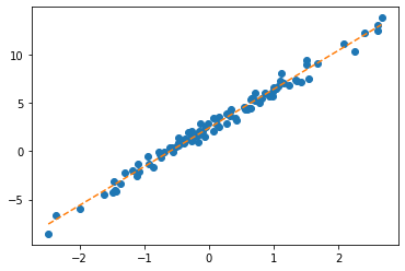

ver2: net = torch.nn.Linear(2,1,bias=False)

- 바로 반복하겠습니다..

net = torch.nn.Linear(2,1,bias=False) 
net.weight.data = torch.tensor([[-5.0, 10.0]])
optimizr = torch.optim.SGD(net.parameters(),lr=1/10) 

plt.plot(x,y,'o')
plt.plot(x,net(X).data,'--')

for epoc in range(30): 
    yhat = net(X)
    loss = torch.mean((y-yhat)**2) 
    loss.backward() 
    optimizr.step(); optimizr.zero_grad() 

plt.plot(x,y,'o')
plt.plot(x,net(X).data,'--')

---

Appendix: net.parameters()의 의미? (선택학습)

- iterator, generator의 개념필요 - https://guebin.github.io/IP2022/2022/06/06/(14주차)-6월6일.html, 클래스공부 8단계 참고

- 탐구시작: 네트워크 생성

net = torch.nn.Linear(in_features=1,out_features=1)
net.weight

Parameter containing:
tensor([[-0.4277]], requires_grad=True)

net.bias

Parameter containing:
tensor([-0.0629], requires_grad=True)

- torch.optim.SGD? 를 확인하면 params에 대한설명에 아래와 같이 되어있음

params (iterable): iterable of parameters to optimize or dicts defining
        parameter groups

- 설명을 읽어보면 params에 iterable object를 넣으라고 되어있음 (iterable object는 숨겨진 명령어로 __iter__를 가지고 있는 오브젝트를 의미)

set(dir(net.parameters)) & {'__iter__'}

set()

set(dir(net.parameters())) & {'__iter__'}

{'__iter__'}

- 무슨의미?

_generator = net.parameters()

_generator.__next__()

Parameter containing:
tensor([[-0.4277]], requires_grad=True)

_generator.__next__()

Parameter containing:
tensor([-0.0629], requires_grad=True)

_generator.__next__()

StopIteration: 

- 이건 이런느낌인데?

_generator2 = iter([net.weight,net.bias])

_generator2

<list_iterator at 0x7f5f0d2cdeb0>

_generator2.__next__()

Parameter containing:
tensor([[-0.4277]], requires_grad=True)

_generator2.__next__()

Parameter containing:
tensor([-0.0629], requires_grad=True)

_generator2.__next__()

StopIteration: 

- 즉 아래는 같은코드이다.

### 코드1
_generator = net.parameters() 
torch.optim.SGD(_generator,lr=1/10) 
### 코드2
_generator = iter([net.weight,net.bias])
torch.optim.SGD(_generator,lr=1/10) 
### 코드3 (이렇게 써도 코드2가 실행된다고 이해할 수 있음)
_iterator = [net.weight,net.bias]
torch.optim.SGD(_iterator,lr=1/10) 

결론: net.parameters()는 net오브젝트에서 학습할 파라메터를 모두 모아 리스트(iterable object)로 만드는 함수라 이해할 수 있다.

- 응용예제1

What = torch.tensor([[-5.0],[10.0]],requires_grad=True)
optimizr = torch.optim.SGD([What],lr=1/10) 

plt.plot(x,y,'o')
plt.plot(x,(X@What).data,'--')

for epoc in range(30):
    yhat = X@What 
    loss = torch.mean((y-yhat)**2)
    loss.backward()
    optimizr.step();optimizr.zero_grad() 

plt.plot(x,y,'o')
plt.plot(x,(X@What).data,'--')

- 응용예제2

b = torch.tensor(-5.0,requires_grad=True)
w = torch.tensor(10.0,requires_grad=True)
optimizr = torch.optim.SGD([b,w],lr=1/10)

plt.plot(x,y,'o')
plt.plot(x,(w*x+b).data,'--')

for epoc in range(30):
    yhat = b+ w*x 
    loss = torch.mean((y-yhat)**2)
    loss.backward()
    optimizr.step(); optimizr.zero_grad()

plt.plot(x,y,'o')
plt.plot(x,(w*x+b).data,'--')

Logistic regression

motive

- 현실에서 이런 경우가 많음 - \(x\)가 커질수록 (혹은 작아질수록) 성공확률이 증가함.

- (X,y)는 어떤모양?

_df = pd.DataFrame({'x':range(-6,7),'y':[0,0,0,0,0,0,1,0,1,1,1,1,1]})
_df 

	x	y
0	-6	0
1	-5	0
2	-4	0
3	-3	0
4	-2	0
5	-1	0
6	0	1
7	1	0
8	2	1
9	3	1
10	4	1
11	5	1
12	6	1

plt.plot(_df.x,_df.y,'o')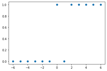

- (예비학습) 시그모이드라는 함수가 있음

xx = torch.linspace(-6,6,100)
def f(x):
    return torch.exp(x)/(1+torch.exp(x))

plt.plot(_df.x,_df.y,'o')
plt.plot(xx,f(xx))
plt.plot(xx,f(2.5*xx-1.2)) # 영향을 크게 받을 때 + 운적인 요소 영향 받을 때(절편) -> 모델링하는 과정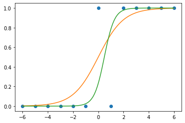

베르누이 특정 확률로 0 또는 1 뽑기

model

- \(x\)가 커질수록 \(y=1\)이 잘나오는 모형은 아래와 같이 설계할 수 있음 <— 외우세요!!!

• \(y_i \sim Ber(\pi_i),\quad\) where \(\pi_i = \frac{\exp(w_0+w_1x_i)}{1+\exp(w_0+w_1x_i)}\)

• \(\hat{y}_i= \hat{pi}_\frac{\exp(\hat{w}_0+\hat{w}_1x_i)}{1+\exp(\hat{w}_0+\hat{w}_1x_i)}=\frac{1}{1+\exp(-\hat{w}_0-\hat{w}_1x_i)}\)

• \(loss= - \sum_{i=1}^{n} \big(y_i\log(\hat{y}_i)+(1-y_i)\log(1-\hat{y}_i)\big)\) <— 외우세요!!

\(y_i=1\) \(\hat{y_i} = 1\)loss가 0 근처 \(\hat{y_i} = 0\) loss가- 무한대

\(y_i = 0\) \(\hat{y_i} = 0\)loss가 0근처 \(\hat{y_i} = 1\) loss가 1

toy example

- 예제시작

torch.bernoulli?

Docstring:
bernoulli(input, *, generator=None, out=None) -> Tensor
Draws binary random numbers (0 or 1) from a Bernoulli distribution.
The :attr:`input` tensor should be a tensor containing probabilities
to be used for drawing the binary random number.
Hence, all values in :attr:`input` have to be in the range:
:math:`0 \leq \text{input}_i \leq 1`.
The :math:`\text{i}^{th}` element of the output tensor will draw a
value :math:`1` according to the :math:`\text{i}^{th}` probability value given
in :attr:`input`.
.. math::
    \text{out}_{i} \sim \mathrm{Bernoulli}(p = \text{input}_{i})
The returned :attr:`out` tensor only has values 0 or 1 and is of the same
shape as :attr:`input`.
:attr:`out` can have integral ``dtype``, but :attr:`input` must have floating
point ``dtype``.
Args:
    input (Tensor): the input tensor of probability values for the Bernoulli distribution
Keyword args:
    generator (:class:`torch.Generator`, optional): a pseudorandom number generator for sampling
    out (Tensor, optional): the output tensor.
Example::
    >>> a = torch.empty(3, 3).uniform_(0, 1)  # generate a uniform random matrix with range [0, 1]
    >>> a
    tensor([[ 0.1737,  0.0950,  0.3609],
            [ 0.7148,  0.0289,  0.2676],
            [ 0.9456,  0.8937,  0.7202]])
    >>> torch.bernoulli(a)
    tensor([[ 1.,  0.,  0.],
            [ 0.,  0.,  0.],
            [ 1.,  1.,  1.]])
    >>> a = torch.ones(3, 3) # probability of drawing "1" is 1
    >>> torch.bernoulli(a)
    tensor([[ 1.,  1.,  1.],
            [ 1.,  1.,  1.],
            [ 1.,  1.,  1.]])
    >>> a = torch.zeros(3, 3) # probability of drawing "1" is 0
    >>> torch.bernoulli(a)
    tensor([[ 0.,  0.,  0.],
            [ 0.,  0.,  0.],
            [ 0.,  0.,  0.]])
Type:      builtin_function_or_method

torch.bernoulli(torch.tensor([0.5]*100)) # 0.5의 확률ㄹ 0 또는 1 뽑아

tensor([0., 1., 0., 1., 0., 0., 1., 0., 0., 0., 0., 1., 0., 1., 1., 0., 1., 1.,
        0., 0., 0., 0., 0., 1., 0., 1., 0., 1., 1., 0., 1., 0., 1., 0., 0., 1.,
        1., 1., 0., 1., 0., 1., 0., 0., 1., 1., 0., 1., 0., 0., 0., 1., 1., 0.,
        1., 0., 0., 0., 0., 0., 0., 1., 0., 0., 0., 0., 1., 1., 1., 0., 0., 0.,
        0., 1., 1., 1., 0., 1., 1., 0., 1., 0., 1., 1., 0., 0., 0., 1., 0., 1.,
        1., 1., 0., 1., 1., 0., 1., 0., 0., 1.])

x=torch.linspace(-1,1,2000).reshape(2000,1)
w0= -1 
w1= 5 
u = w0+x*w1 
v = torch.exp(u)/(1+torch.exp(u)) # v=πi, 즉 확률을 의미함
y = torch.bernoulli(v) 

v

tensor([[0.0025],
        [0.0025],
        [0.0025],
        ...,
        [0.9818],
        [0.9819],
        [0.9820]])

u

tensor([[-6.0000],
        [-5.9950],
        [-5.9900],
        ...,
        [ 3.9900],
        [ 3.9950],
        [ 4.0000]])

#plt.scatter(x,y,alpha=0.05)
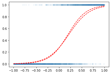
plt.plot(x,y,'o',alpha=0.05,ms=4)
plt.plot(x,v,'--r')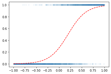

• 우리의 목적: \(x\)가 들어가면 빨간선 \(\hat{y}\)의 값을 만들어주는 mapping을 학습해보자.

w0hat = 10
w1hat = 3
yhat = f(w0hat + w1hat*x)
plt.plot(x,y,'o',alpha=0.05,ms=4)
plt.plot(x,v,'--r')
plt.plot(x,yhat,'--r')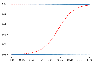

l1 = torch.nn.Linear(1,1)

l1.bias.data = torch.tensor([-1.0])
l1.weight.data = torch.tensor([[1.0]])

a1 = torch.nn.Sigmoid()

w0hat = -1
w1hat = 3
yhat = a1(w0hat + w1hat*x)
plt.plot(x,y,'o',alpha=0.05,ms=4)
plt.plot(x,v,'--r')
plt.plot(x,yhat,'--r')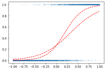

for epoc in range(6000):
    ## step1 
    yhat = a1(l1(x))
    ## step2 
    loss = torch.mean((y-yhat)**2) ## loss 를 원래 이렇게 하는건 아니에요.. 
    ## step3 
    loss.backward()
    ## step4 
    l1.bias.data = l1.bias.data - 0.1 * l1.bias.grad 
    l1.weight.data = l1.weight.data - 0.1 * l1.weight.grad 
    l1.bias.grad = None 
    l1.weight.grad = None 

plt.plot(x,y,'o',alpha=0.05,ms=4)
plt.plot(x,v,'--r')
plt.plot(x,a1(l1(x)).data,'--r')

---

숙제