순환신경망 minor topics

imports

import torch
import pandas as pd
import matplotlib.pyplot as plt 
from fastai.text.all import *
import pytorch_lightning as pl

Define some funtions

def f(txt,mapping):
    return [mapping[key] for key in txt] 
sig = torch.nn.Sigmoid()
soft = torch.nn.Softmax(dim=1)
tanh = torch.nn.Tanh()

순환신경망 표현력 비교실험 (1)

data: abcabC

txt = list('abcabC')*100
txt[:8]
txt_x = txt[:-1] 
txt_y = txt[1:]

mapping = {'a':0,'b':1,'c':2,'C':3} 
x= torch.nn.functional.one_hot(torch.tensor(f(txt_x,mapping))).float()
y= torch.nn.functional.one_hot(torch.tensor(f(txt_y,mapping))).float()

x = x.to("cuda:0")
y = y.to("cuda:0")

x.shape

torch.Size([599, 4])

실험

- 실험1

HIDDEN = 3

fig, ax = plt.subplots(5,5,figsize=(10,10))
for i in range(5):
    for j in range(5):
        rnn = torch.nn.RNN(4,HIDDEN).to("cuda:0")
        linr = torch.nn.Linear(HIDDEN,4).to("cuda:0")
        loss_fn = torch.nn.CrossEntropyLoss()
        optimizr = torch.optim.Adam(list(rnn.parameters())+list(linr.parameters()),lr=0.1)
        _water = torch.zeros(1,HIDDEN).to("cuda:0")
        for epoc in range(500):
            ## 1
            hidden, hT = rnn(x,_water)
            output = linr(hidden)
            ## 2
            loss = loss_fn(output,y)
            ## 3
            loss.backward()
            ## 4 
            optimizr.step()
            optimizr.zero_grad()
        yhat=soft(output)    
        combind = torch.concat([hidden,yhat],axis=1)
        ax[i][j].matshow(combind.to("cpu").data[-6:],cmap='bwr',vmin=-1,vmax=1)
fig.suptitle("experiment1: RNN with {} hidden nodes".format(HIDDEN),size=20)
fig.tight_layout()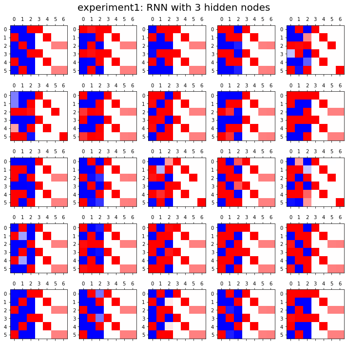

- 실험2

HIDDEN = 4

fig, ax = plt.subplots(5,5,figsize=(10,10))
for i in range(5):
    for j in range(5):
        rnn = torch.nn.RNN(4,HIDDEN).to("cuda:0")
        linr = torch.nn.Linear(HIDDEN,4).to("cuda:0")
        loss_fn = torch.nn.CrossEntropyLoss()
        optimizr = torch.optim.Adam(list(rnn.parameters())+list(linr.parameters()),lr=0.1)
        _water = torch.zeros(1,HIDDEN).to("cuda:0")
        for epoc in range(500):
            ## 1
            hidden, hT = rnn(x,_water)
            output = linr(hidden)
            ## 2
            loss = loss_fn(output,y)
            ## 3
            loss.backward()
            ## 4 
            optimizr.step()
            optimizr.zero_grad()
        yhat=soft(output)    
        combind = torch.concat([hidden,yhat],axis=1)
        ax[i][j].matshow(combind.to("cpu").data[-6:],cmap='bwr',vmin=-1,vmax=1)
fig.suptitle("experiment2: RNN with {} hidden nodes".format(HIDDEN),size=20)
fig.tight_layout()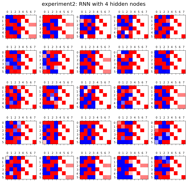

- 실험3

HIDDEN = 8

fig, ax = plt.subplots(5,5,figsize=(10,8))
for i in range(5):
    for j in range(5):
        rnn = torch.nn.RNN(4,HIDDEN).to("cuda:0")
        linr = torch.nn.Linear(HIDDEN,4).to("cuda:0")
        loss_fn = torch.nn.CrossEntropyLoss()
        optimizr = torch.optim.Adam(list(rnn.parameters())+list(linr.parameters()),lr=0.1)
        _water = torch.zeros(1,HIDDEN).to("cuda:0")
        for epoc in range(500):
            ## 1
            hidden, hT = rnn(x,_water)
            output = linr(hidden)
            ## 2
            loss = loss_fn(output,y)
            ## 3
            loss.backward()
            ## 4 
            optimizr.step()
            optimizr.zero_grad()
        yhat=soft(output)    
        combind = torch.concat([hidden,yhat],axis=1)
        ax[i][j].matshow(combind.to("cpu").data[-6:],cmap='bwr',vmin=-1,vmax=1)
fig.suptitle("experiment3: RNN with {} hidden nodes".format(HIDDEN),size=20)
fig.tight_layout()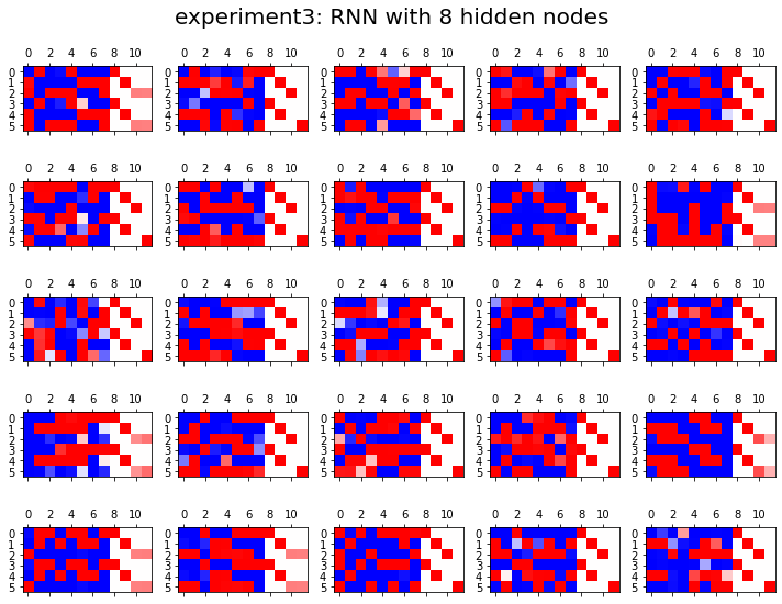

결론

- 노드수가 많으면 학습에 유리함

(서연 필기) c/C를 맞추는 것(error)보다 확실한 규칙을 맞추는 것(underline)이 중요\(\to\)오히려 맞추면 과적합으로 볼 수 있다 - 그래서 학습이 잘 되었으면 - 첫 칸 - 둘째 칸 - 셋쨰, 넷째 칸 - 이 순으로 predict 되었을 것

순환신경망 표현력 비교실험 (2)

data: ab(c,C)

# torch.manual_seed(43052)
# txta = 'a'*50
# txtb = 'b'*50
# prob_upper = torch.bernoulli(torch.zeros(50)+0.5) 
# txtc = list(map(lambda x: 'c' if x==1 else 'C', prob_upper))
# txt = ''.join([txta[i]+','+txtb[i]+','+txtc[i]+',' for i in range(50)]).split(',')[:-1]
# txt_x = txt[:-1] 
# txt_y = txt[1:]
# pd.DataFrame({'txt_x':txt_x,'txt_y':txt_y}).to_csv("2022-11-25-ab(c,C).csv",index=False)

df= pd.read_csv("https://raw.githubusercontent.com/guebin/DL2022/main/posts/IV.%20RNN/2022-11-25-ab(c%2CC).csv")
df

	txt_x	txt_y
0	a	b
1	b	c
2	c	a
3	a	b
4	b	c
...	...	...
144	a	b
145	b	C
146	C	a
147	a	b
148	b	c

149 rows × 2 columns

mapping = {'a':0,'b':1,'c':2,'C':3} 
x= torch.nn.functional.one_hot(torch.tensor(f(df.txt_x,mapping))).float()
y= torch.nn.functional.one_hot(torch.tensor(f(df.txt_y,mapping))).float()

x = x.to("cuda:0")
y = y.to("cuda:0")

실험

- 실험1

HIDDEN = 3

fig, ax = plt.subplots(5,5,figsize=(10,10))
for i in range(5):
    for j in range(5):
        lstm = torch.nn.LSTM(4,HIDDEN).to("cuda:0")
        linr = torch.nn.Linear(HIDDEN,4).to("cuda:0")
        loss_fn = torch.nn.CrossEntropyLoss()
        optimizr = torch.optim.Adam(list(lstm.parameters())+list(linr.parameters()),lr=0.1)
        _water = torch.zeros(1,HIDDEN).to("cuda:0")
        for epoc in range(500):
            ## 1
            hidden, (hT,cT) = lstm(x,(_water,_water))
            output = linr(hidden)
            ## 2
            loss = loss_fn(output,y)
            ## 3
            loss.backward()
            ## 4 
            optimizr.step()
            optimizr.zero_grad()
        yhat=soft(output)    
        combinded = torch.concat([yhat,y],axis=1)
        ax[i][j].matshow(combinded.to("cpu").data[-6:],cmap='bwr',vmin=-1,vmax=1)
fig.suptitle("experiment1: LSTM with {} hidden nodes".format(HIDDEN),size=20)
fig.tight_layout()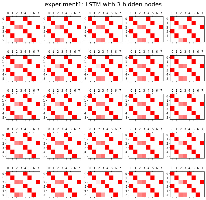

- 실험2

HIDDEN = 16

fig, ax = plt.subplots(5,5,figsize=(10,10))
for i in range(5):
    for j in range(5):
        lstm = torch.nn.LSTM(4,HIDDEN).to("cuda:0")
        linr = torch.nn.Linear(HIDDEN,4).to("cuda:0")
        loss_fn = torch.nn.CrossEntropyLoss()
        optimizr = torch.optim.Adam(list(lstm.parameters())+list(linr.parameters()),lr=0.1)
        _water = torch.zeros(1,HIDDEN).to("cuda:0")
        for epoc in range(500):
            ## 1
            hidden, (hT,cT) = lstm(x,(_water,_water))
            output = linr(hidden)
            ## 2
            loss = loss_fn(output,y)
            ## 3
            loss.backward()
            ## 4 
            optimizr.step()
            optimizr.zero_grad()
        yhat=soft(output)    
        combinded = torch.concat([yhat,y],axis=1)
        ax[i][j].matshow(combinded.to("cpu").data[-6:],cmap='bwr',vmin=-1,vmax=1)
fig.suptitle("experiment2: LSTM with {} hidden nodes".format(HIDDEN),size=20)
fig.tight_layout()

결론

- 노드수가 너무 많으면 오버피팅 경향도 있음

문자열에서 단어로

data: human numbers 5

txt = (['one',',','two',',','three',',','four',',','five',',']*100)[:-1]

mapping = {',':0, 'one':1, 'two':2, 'three':3, 'four':4, 'five':5} 
mapping

{',': 0, 'one': 1, 'two': 2, 'three': 3, 'four': 4, 'five': 5}

txt_x = txt[:-1]
txt_y = txt[1:]

txt_x[0:5], txt_y[0:5]

(['one', ',', 'two', ',', 'three'], [',', 'two', ',', 'three', ','])

x = torch.nn.functional.one_hot(torch.tensor(f(txt_x,mapping))).float().to("cuda:0")
y = torch.nn.functional.one_hot(torch.tensor(f(txt_y,mapping))).float().to("cuda:0")

torch를 이용한 learn

torch.manual_seed(43052) 
lstm = torch.nn.LSTM(6,20).to("cuda:0") 
linr = torch.nn.Linear(20,6).to("cuda:0") 
loss_fn = torch.nn.CrossEntropyLoss()
optimizr = torch.optim.Adam(list(lstm.parameters())+list(linr.parameters()),lr=0.1)

_water = torch.zeros(1,20).to("cuda:0")
for epoc in range(50):
    ## 1 
    hidden, (hT,cT) =lstm(x,(_water,_water))
    output = linr(hidden) 
    ## 2 
    loss = loss_fn(output,y) 
    ## 3 
    loss.backward()
    ## 4 
    optimizr.step()
    optimizr.zero_grad()

plt.matshow(soft(output).data[-10:].to("cpu"),cmap='bwr',vmin=-1,vmax=1)

fastai 이용한 learn

ds1 = torch.utils.data.TensorDataset(x,y)
ds2 = torch.utils.data.TensorDataset(x,y) # dummy 
dl1 = torch.utils.data.DataLoader(ds1,batch_size=998)
dl2 = torch.utils.data.DataLoader(ds2,batch_size=998) # dummy 
dls = DataLoaders(dl1,dl2)

fastai 를 이용하여 class를 사용하기 위한 목차

class MyLSTM(torch.nn.Module):
    def __init__(self):
        super().__init__()
        self.lstm = torch.nn.LSTM(6,20)
        self.linr = torch.nn.Linear(20,6) 
    def forward(self,x):
        _water = torch.zeros(1,20).to("cuda:0")
        hidden, (hT,cT) =self.lstm(x,(_water,_water))
        output = self.linr(hidden)
        return output

net = MyLSTM().to("cuda:0")
loss_fn = torch.nn.CrossEntropyLoss()

lrnr = Learner(dls,net,loss_fn,lr=0.1)

lrnr.fit(50)

epoch	train_loss	valid_loss	time
0	1.722138	1.502271	00:00
1	1.611093	1.973368	00:00
2	1.734299	1.481888	00:00
3	1.669271	1.377668	00:00
4	1.608570	1.368541	00:00
5	1.566517	1.267919	00:00
6	1.521232	1.106543	00:00
7	1.465657	0.959904	00:00
8	1.404815	0.856123	00:00
9	1.344825	0.802936	00:00
10	1.290437	0.794831	00:00
11	1.244395	0.771966	00:00
12	1.203488	0.735865	00:00
13	1.165525	0.690032	00:00
14	1.129149	0.621654	00:00
15	1.092401	0.555875	00:00
16	1.055485	0.493046	00:00
17	1.018588	0.423167	00:00
18	0.981230	0.349703	00:00
19	0.943231	0.279531	00:00
20	0.904838	0.216544	00:00
21	0.866475	0.166756	00:00
22	0.828821	0.125583	00:00
23	0.792214	0.094763	00:00
24	0.757037	0.072662	00:00
25	0.723539	0.055544	00:00
26	0.691763	0.042442	00:00
27	0.661703	0.032804	00:00
28	0.633335	0.025908	00:00
29	0.606606	0.020872	00:00
30	0.581437	0.017020	00:00
31	0.557727	0.014002	00:00
32	0.535379	0.011625	00:00
33	0.514297	0.009755	00:00
34	0.494391	0.008293	00:00
35	0.475579	0.007180	00:00
36	0.457784	0.006386	00:00
37	0.440938	0.005807	00:00
38	0.424976	0.005199	00:00
39	0.409830	0.004525	00:00
40	0.395437	0.003926	00:00
41	0.381747	0.003398	00:00
42	0.368712	0.002977	00:00
43	0.356291	0.002673	00:00
44	0.344447	0.002432	00:00
45	0.333144	0.002230	00:00
46	0.322349	0.002058	00:00
47	0.312030	0.001911	00:00
48	0.302160	0.001785	00:00
49	0.292712	0.001678	00:00

plt.matshow(soft(lrnr.model(x)[-10:]).data.to("cpu"),cmap = 'bwr', vmin=-1,vmax=1)

똑같은 코드들: `torch.nn.LSTM`

data: hi?hello!!

txt = list('hi?hello!!')*100 
txt_x = txt[:-1]
txt_y = txt[1:]

mapping = {'!':0, '?':1,'h':2,'i':3,'e':4,'l':5,'o':6} 
x= torch.nn.functional.one_hot(torch.tensor(f(txt_x,mapping))).float().to("cuda:0")
y= torch.nn.functional.one_hot(torch.tensor(f(txt_y,mapping))).float().to("cuda:0")

세트1: _water의 생략

- 코드1: 정석코드

torch.manual_seed(43052)
lstm = torch.nn.LSTM(7,4).to("cuda:0")

_water = torch.zeros(1,4).to("cuda:0")
lstm(x, (_water,_water))

(tensor([[-0.1547,  0.0673,  0.0695,  0.1563],
         [-0.0786, -0.1430, -0.0250,  0.1189],
         [-0.0300, -0.2256, -0.1324,  0.1439],
         ...,
         [-0.0723,  0.0620,  0.1913,  0.2015],
         [-0.1155,  0.0746,  0.1747,  0.2938],
         [-0.2350, -0.1559, -0.1093,  0.2682]], device='cuda:0',
        grad_fn=<SqueezeBackward1>),
 (tensor([[-0.2350, -0.1559, -0.1093,  0.2682]], device='cuda:0',
         grad_fn=<SqueezeBackward1>),
  tensor([[-0.4451, -0.2456, -0.1900,  0.6232]], device='cuda:0',
         grad_fn=<SqueezeBackward1>)))

- 코드2: _water 는 사실 없어도 괜찮았어..

torch.manual_seed(43052)
lstm = torch.nn.LSTM(7,4).to("cuda:0")

lstm(x)

(tensor([[-0.1547,  0.0673,  0.0695,  0.1563],
         [-0.0786, -0.1430, -0.0250,  0.1189],
         [-0.0300, -0.2256, -0.1324,  0.1439],
         ...,
         [-0.0723,  0.0620,  0.1913,  0.2015],
         [-0.1155,  0.0746,  0.1747,  0.2938],
         [-0.2350, -0.1559, -0.1093,  0.2682]], device='cuda:0',
        grad_fn=<SqueezeBackward1>),
 (tensor([[-0.2350, -0.1559, -0.1093,  0.2682]], device='cuda:0',
         grad_fn=<SqueezeBackward1>),
  tensor([[-0.4451, -0.2456, -0.1900,  0.6232]], device='cuda:0',
         grad_fn=<SqueezeBackward1>)))

x.shape

torch.Size([999, 7])

999개, 구별되는 문자 7개

세트2: x.shape = (\(L\), \(H_{in}\)) or (\(L\),\(N\),\(H_{in}\))

- 파라메터 설명

\(L\) = sequece length = 시계열의 길이 = 간장을 몇 년 전통으로 이어갈지
\(N\) = batch size = 전체데이터는 몇 개의 시계열이 있는지 = 전체 데이터를 몇개의 시계열로 쪼갤지 <– 왜 이걸 해야해?
\(H_{in}\) = input_size = 시점을 고정하였을 경우 입력자료의 차원 = 입력시계열이 시점별로 몇개의 변수로 나타내어 지는지? = 만약에 원핫인코딩으로 단어를 정리하면 단어수를 의미함

우리가 실습했던 거 모두 N이 1이었다 그래서 안 썼음 - 1일 때만 아래와 같이 여러 버전 가능

- 코드2: _water 는 사실 없어도 괜찮았어..

torch.manual_seed(43052)
lstm = torch.nn.LSTM(7,4).to("cuda:0")

lstm(x)

(tensor([[-0.1547,  0.0673,  0.0695,  0.1563],
         [-0.0786, -0.1430, -0.0250,  0.1189],
         [-0.0300, -0.2256, -0.1324,  0.1439],
         ...,
         [-0.0723,  0.0620,  0.1913,  0.2015],
         [-0.1155,  0.0746,  0.1747,  0.2938],
         [-0.2350, -0.1559, -0.1093,  0.2682]], device='cuda:0',
        grad_fn=<SqueezeBackward1>),
 (tensor([[-0.2350, -0.1559, -0.1093,  0.2682]], device='cuda:0',
         grad_fn=<SqueezeBackward1>),
  tensor([[-0.4451, -0.2456, -0.1900,  0.6232]], device='cuda:0',
         grad_fn=<SqueezeBackward1>)))

- 코드3: x의 차원은 사실 엄밀하게는 (\(L\),\(N\),\(H_{in}\)) 와 같다…

torch.manual_seed(43052)
lstm = torch.nn.LSTM(7,4).to("cuda:0")

lstm(x.reshape(999,1,7))

(tensor([[[-0.1547,  0.0673,  0.0695,  0.1563]],
 
         [[-0.0786, -0.1430, -0.0250,  0.1189]],
 
         [[-0.0300, -0.2256, -0.1324,  0.1439]],
 
         ...,
 
         [[-0.0723,  0.0620,  0.1913,  0.2015]],
 
         [[-0.1155,  0.0746,  0.1747,  0.2938]],
 
         [[-0.2350, -0.1559, -0.1093,  0.2682]]], device='cuda:0',
        grad_fn=<CudnnRnnBackward0>),
 (tensor([[[-0.2350, -0.1559, -0.1093,  0.2682]]], device='cuda:0',
         grad_fn=<CudnnRnnBackward0>),
  tensor([[[-0.4451, -0.2456, -0.1900,  0.6232]]], device='cuda:0',
         grad_fn=<CudnnRnnBackward0>)))

- 코드4: batch_first=True옵션을 사용하여 lstm을 만든경우

torch.manual_seed(43052)
lstm = torch.nn.LSTM(7,4,batch_first=True).to("cuda:0")

lstm(x.reshape(1,999,7))

(tensor([[[-0.1547,  0.0673,  0.0695,  0.1563],
          [-0.0786, -0.1430, -0.0250,  0.1189],
          [-0.0300, -0.2256, -0.1324,  0.1439],
          ...,
          [-0.0723,  0.0620,  0.1913,  0.2015],
          [-0.1155,  0.0746,  0.1747,  0.2938],
          [-0.2350, -0.1559, -0.1093,  0.2682]]], device='cuda:0',
        grad_fn=<CudnnRnnBackward0>),
 (tensor([[[-0.2350, -0.1559, -0.1093,  0.2682]]], device='cuda:0',
         grad_fn=<CudnnRnnBackward0>),
  tensor([[[-0.4451, -0.2456, -0.1900,  0.6232]]], device='cuda:0',
         grad_fn=<CudnnRnnBackward0>)))

세트3: hidden.shape = (\(D\times\) `num_layers`, \(H_{out}\)) or (\(D\times\) `num_layers`, \(N\), \(H_{out}\))

- 파라메터 설명

\(D\) = 2 if bidirectional=True otherwise 1 = 양방향이면 2, 단방향이면 1 (우리는 단방향만 배움)
num_layres = 중첩된 RNN일 경우 (우리는 중첩을 안시켰음)
\(N\) = batch size = 전체데이터는 몇 개의 시계열이 있는지 = 전체 데이터를 몇개의 시계열로 쪼갤지 <– 왜 이걸 해야해?
\(H_{out}\) = 히든노드의 수

- 코드5: x.shape = (\(L\),\(1\),\(H_{in}\)) \(\to\) hidden.shape = (\(1\),\(1\),\(H_{out}\))

torch.manual_seed(43052)
lstm = torch.nn.LSTM(7,4).to("cuda:0")

_water = torch.zeros(1,1,4).to("cuda:0") 
lstm(x.reshape(999,1,7),(_water,_water))

(tensor([[[-0.1547,  0.0673,  0.0695,  0.1563]],
 
         [[-0.0786, -0.1430, -0.0250,  0.1189]],
 
         [[-0.0300, -0.2256, -0.1324,  0.1439]],
 
         ...,
 
         [[-0.0723,  0.0620,  0.1913,  0.2015]],
 
         [[-0.1155,  0.0746,  0.1747,  0.2938]],
 
         [[-0.2350, -0.1559, -0.1093,  0.2682]]], device='cuda:0',
        grad_fn=<CudnnRnnBackward0>),
 (tensor([[[-0.2350, -0.1559, -0.1093,  0.2682]]], device='cuda:0',
         grad_fn=<CudnnRnnBackward0>),
  tensor([[[-0.4451, -0.2456, -0.1900,  0.6232]]], device='cuda:0',
         grad_fn=<CudnnRnnBackward0>)))

- 사실 _water.shape = (1,\(H_{out}\)) 에서 1은 observation의 차원을 의미하는게 아님 (그런데 대충 그렇게 생각해도 무방함)

한 시점의 콩물에 대하여 양방향으로 간장을 만들면 _water.shape = (2,h)
한 시점의 콩물에 대하여 3중첩으로 간장을 만들면 _water.shape = (3,h)
한 시점의 콩물에 대하여 3중첩간장을 양방향으로 만들면 _water.shape = (6,h)

똑같은 코드들: `torch.nn.LSTMCell`

data: hi?hello!!

txt = list('hi?hello!!')*100 
txt_x = txt[:-1]
txt_y = txt[1:]

mapping = {'!':0, '?':1,'h':2,'i':3,'e':4,'l':5,'o':6} 
x= torch.nn.functional.one_hot(torch.tensor(f(txt_x,mapping))).float().to("cuda:0")
y= torch.nn.functional.one_hot(torch.tensor(f(txt_y,mapping))).float().to("cuda:0")

세트1: _water의 생략

- 코드1: 정석코드

torch.manual_seed(43052) 
lstmcell = torch.nn.LSTMCell(7,4).to("cuda:0")

xt = x[[1]]
_water = torch.zeros(1,4).to("cuda:0")
xt.shape, _water.shape

(torch.Size([1, 7]), torch.Size([1, 4]))

lstmcell(xt,(_water,_water))

(tensor([[-0.0290, -0.1758, -0.0537,  0.0598]], device='cuda:0',
        grad_fn=<ThnnFusedLstmCellBackward0>),
 tensor([[-0.0582, -0.4566, -0.1256,  0.1922]], device='cuda:0',
        grad_fn=<ThnnFusedLstmCellBackward0>))

- 코드2: _water의 생략

torch.manual_seed(43052) 
lstmcell = torch.nn.LSTMCell(7,4).to("cuda:0")

xt = x[[1]]
xt.shape

torch.Size([1, 7])

lstmcell(xt)

(tensor([[-0.0290, -0.1758, -0.0537,  0.0598]], device='cuda:0',
        grad_fn=<ThnnFusedLstmCellBackward0>),
 tensor([[-0.0582, -0.4566, -0.1256,  0.1922]], device='cuda:0',
        grad_fn=<ThnnFusedLstmCellBackward0>))

세트2: xt.shape = (\(N\),\(H_{in}\)) or (\(H_{in}\))

n: timeserie 개수, 1일 경우 생략 가능

- 코드2: _water의 생략

torch.manual_seed(43052) 
lstmcell = torch.nn.LSTMCell(7,4).to("cuda:0")

xt = x[[1]]
xt.shape

torch.Size([1, 7])

lstmcell(xt)

(tensor([[-0.0290, -0.1758, -0.0537,  0.0598]], device='cuda:0',
        grad_fn=<ThnnFusedLstmCellBackward0>),
 tensor([[-0.0582, -0.4566, -0.1256,  0.1922]], device='cuda:0',
        grad_fn=<ThnnFusedLstmCellBackward0>))

- 코드3:

torch.manual_seed(43052) 
lstmcell = torch.nn.LSTMCell(7,4).to("cuda:0")

xt = x[1]
xt.shape

torch.Size([7])

lstmcell(xt)

(tensor([-0.0290, -0.1758, -0.0537,  0.0598], device='cuda:0',
        grad_fn=<SqueezeBackward1>),
 tensor([-0.0582, -0.4566, -0.1256,  0.1922], device='cuda:0',
        grad_fn=<SqueezeBackward1>))

(1,n)의 형태라면 괄호 하나 빼도 가능

세트3: hidden.shape = (\(N\),\(H_{out}\)) or (\(H_{out}\))

- 코드4: xt.shape = (\(H_{out}\)) \(\to\) _water.shape = \((H_{out})\)

torch.manual_seed(43052) 
lstmcell = torch.nn.LSTMCell(7,4).to("cuda:0")

xt = x[1]
_water = torch.zeros(4).to("cuda:0")
xt.shape,_water.shape

(torch.Size([7]), torch.Size([4]))

lstmcell(xt, (_water,_water))

(tensor([-0.0290, -0.1758, -0.0537,  0.0598], device='cuda:0',
        grad_fn=<SqueezeBackward1>),
 tensor([-0.0582, -0.4566, -0.1256,  0.1922], device='cuda:0',
        grad_fn=<SqueezeBackward1>))

Summary

똑같은 코드들 정리

- 원래 1은 단순히 observation의 차원이 아니다. 즉 \({\bf X}_{n \times p}\)에서 \(n\)에 대응하는 차원으로 생각할 수 없다.

- 그런데 (1) 단방향 (2) 조각내지 않은 시계열 (3) 중첩하지 않은 순환망에 한정하여서는 observation 처럼 생각해도 무방하다. <– 엄밀하게는 이게 위험한 생각임. 하지만 정식으로 모두 따지려면 너무 헷갈림

실제구현시 기억할 것

- 현실적으로 (1)-(3)이 아닌 조건에서는 Cell 단위로 연산을 이용할 일이 없다. (느리거든요) // 그냥 이해용으로 구현

- torch.nn.RNN 혹은 torch.nn.LSTM 으로 네트워크를 구성할시 _water의 dim을 명시할 일도 없다.

- 오로지 고려해야 할 것은 입력시계열을 조각낼지 조각내지 않을지

조각난 시계열로 학습

시계열이 무조건 연속으로서 데이터가 존재하지 않는다면? - 댓글 1의 길이는 400 - 댓글 2 의 길이는 100 이럴수도

data

txt = list('hi!')*3 + list('hi?')*3

조각내지 않은 시계열

txt_x = txt[:-1] 
txt_y = txt[1:]

mapping = {'!':0, '?':1, 'h':2, 'i':3} 
x = torch.nn.functional.one_hot(torch.tensor(f(txt_x,mapping))).float().to("cuda:0")
y = torch.nn.functional.one_hot(torch.tensor(f(txt_y,mapping))).float().to("cuda:0")

torch.manual_seed(43052) 
lstm = torch.nn.LSTM(4,10).to("cuda:0")
linr = torch.nn.Linear(10,4).to("cuda:0")

loss_fn = torch.nn.CrossEntropyLoss() 
optimizr = torch.optim.Adam(list(lstm.parameters())+list(linr.parameters()),lr=0.1)

for epoc in range(100):
    ## 1 
    hidden, _ = lstm(x) 
    output = linr(hidden) 
    ## 2 
    loss = loss_fn(output,y) 
    ## 3 
    loss.backward() 
    ## 4 
    optimizr.step()
    optimizr.zero_grad()

hidden, _ = lstm(x)
plt.matshow(soft(linr(hidden)).to("cpu").data,cmap='bwr',vmin=-1,vmax=1)

첫번째 stack은 hi!로 학습 두번째 stack은 hi?로 학습하여 결과가 이럼

조각난 시계열

txt1= txt[:9]
txt2= txt[9:]

txt1,txt2

(['h', 'i', '!', 'h', 'i', '!', 'h', 'i', '!'],
 ['h', 'i', '?', 'h', 'i', '?', 'h', 'i', '?'])

txt1_x = txt1[:-1] 
txt1_y = txt1[1:] 
txt2_x = txt2[:-1] 
txt2_y = txt2[1:]

mapping = {'!':0, '?':1, 'h':2, 'i':3} 
x1 = torch.nn.functional.one_hot(torch.tensor(f(txt1_x,mapping))).float().to("cuda:0")
y1 = torch.nn.functional.one_hot(torch.tensor(f(txt1_y,mapping))).float().to("cuda:0")
x2 = torch.nn.functional.one_hot(torch.tensor(f(txt2_x,mapping))).float().to("cuda:0")
y2 = torch.nn.functional.one_hot(torch.tensor(f(txt2_y,mapping))).float().to("cuda:0")

9에서 하나씩 빼서 x,y 만들었으니까 8

x1.shape, y1.shape, x2.shape, y2.shape

(torch.Size([8, 4]),
 torch.Size([8, 4]),
 torch.Size([8, 4]),
 torch.Size([8, 4]))

xx = torch.stack([x1,x2],axis=1)
yy = torch.stack([y1,y2],axis=1)
xx.shape, yy.shape

(torch.Size([8, 2, 4]), torch.Size([8, 2, 4]))

torch.manual_seed(43052) 
lstm = torch.nn.LSTM(4,10).to("cuda:0")
linr = torch.nn.Linear(10,4).to("cuda:0")

loss_fn = torch.nn.CrossEntropyLoss() 
optimizr = torch.optim.Adam(list(lstm.parameters())+list(linr.parameters()),lr=0.1)

for epoc in range(100):
    ## 1 
    hidden, _ = lstm(xx) 
    output = linr(hidden) 
    ## 2 
    loss = loss_fn(output[:,0,:],yy[:,0,:]) + loss_fn(output[:,1,:],yy[:,1,:])
    ## 3 
    loss.backward() 
    ## 4 
    optimizr.step()
    optimizr.zero_grad()

첫번째 stzck 과 두번째 stack의 합

  loss = loss_fn(output[:,0,:],yy[:,0,:]) + loss_fn(output[:,1,:],yy[:,1,:])

fig , ax = plt.subplots(1,2) 
ax[0].matshow(soft(output[:,0,:]).to("cpu").data,cmap='bwr',vmin=-1,vmax=1)
ax[1].matshow(soft(output[:,1,:]).to("cpu").data,cmap='bwr',vmin=-1,vmax=1)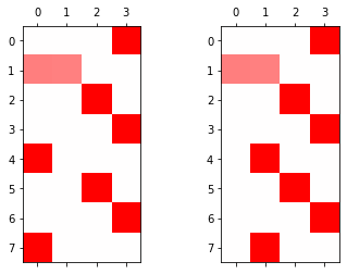

xx로 학습한 것들인데 만약 x를 넣는다면?

hidden, _ = lstm(x)
plt.matshow(soft(linr(hidden)).to("cpu").data,cmap='bwr',vmin=-1,vmax=1)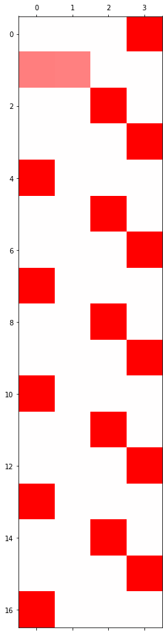

hidden, _ = lstm(x1)
plt.matshow(soft(linr(hidden)).to("cpu").data,cmap='bwr',vmin=-1,vmax=1)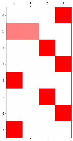

hidden, _ = lstm(x2)
plt.matshow(soft(linr(hidden)).to("cpu").data,cmap='bwr',vmin=-1,vmax=1)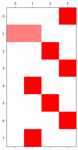

hidden.shape

torch.Size([17, 10])

linr(hidden).shape

torch.Size([17, 4])

- 조각난 시계열로 학습한 경우는 hi!에서 hi?로 바뀔 수 없다. 왜냐햐면 그러한 연결정보가 끊어져 있으니까

재미있는 실험

- x1만 배운다면?

torch.manual_seed(43052) 
lstm = torch.nn.LSTM(4,10).to("cuda:0")
linr = torch.nn.Linear(10,4).to("cuda:0")

loss_fn = torch.nn.CrossEntropyLoss() 
optimizr = torch.optim.Adam(list(lstm.parameters())+list(linr.parameters()),lr=0.1)

for epoc in range(100):
    ## 1 
    hidden, _ = lstm(x1) 
    output = linr(hidden) 
    ## 2 
    loss = loss_fn(output,y1)
    ## 3 
    loss.backward() 
    ## 4 
    optimizr.step()
    optimizr.zero_grad()

hidden, _ = lstm(x2)
plt.matshow(soft(linr(hidden)).to("cpu").data,cmap='bwr',vmin=-1,vmax=1)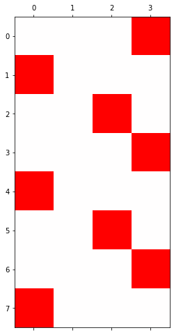

- x2만 배운다면?

torch.manual_seed(43052) 
lstm = torch.nn.LSTM(4,10).to("cuda:0")
linr = torch.nn.Linear(10,4).to("cuda:0")

loss_fn = torch.nn.CrossEntropyLoss() 
optimizr = torch.optim.Adam(list(lstm.parameters())+list(linr.parameters()),lr=0.1)

for epoc in range(100):
    ## 1 
    hidden, _ = lstm(x2) 
    output = linr(hidden) 
    ## 2 
    loss = loss_fn(output,y2)
    ## 3 
    loss.backward() 
    ## 4 
    optimizr.step()
    optimizr.zero_grad()

hidden, _ = lstm(x1)
plt.matshow(soft(linr(hidden)).to("cpu").data,cmap='bwr',vmin=-1,vmax=1)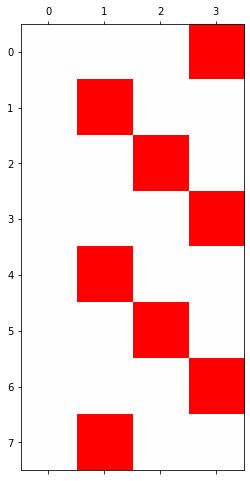

똑같은 코드들 fastai, pytorch

data: human numbers 5

txt = (['one',',','two',',','three',',','four',',','five',',']*100)[:-1]

mapping = {',':0, 'one':1, 'two':2, 'three':3, 'four':4, 'five':5} 
mapping

{',': 0, 'one': 1, 'two': 2, 'three': 3, 'four': 4, 'five': 5}

txt_x = txt[:-1]
txt_y = txt[1:]

txt_x[0:5], txt_y[0:5]

(['one', ',', 'two', ',', 'three'], [',', 'two', ',', 'three', ','])

x = torch.nn.functional.one_hot(torch.tensor(f(txt_x,mapping))).float().to("cuda:0")
y = torch.nn.functional.one_hot(torch.tensor(f(txt_y,mapping))).float().to("cuda:0")

fastai 이용한 learn

dl1 = torch.utils.data.DataLoader(ds1,batch_size=998)

한 뭉치에 몇 개 있는지

torch.nn.LSTM(batxh_size)

몇 개로 나눠져 있는지

ds1 = torch.utils.data.TensorDataset(x,y)
ds2 = torch.utils.data.TensorDataset(x,y) # dummy 
dl1 = torch.utils.data.DataLoader(ds1,batch_size=998)
dl2 = torch.utils.data.DataLoader(ds2,batch_size=998) # dummy 
dls = DataLoaders(dl1,dl2)

class MyLSTM(torch.nn.Module):
    def __init__(self):
        super().__init__()
        torch.manual_seed(43052)
        self.lstm = torch.nn.LSTM(6,20)
        self.linr = torch.nn.Linear(20,6) 
    def forward(self,x):
        _water = torch.zeros(1,20).to("cuda:0")
        hidden, (hT,cT) =self.lstm(x,(_water,_water))
        output = self.linr(hidden)
        return output

net = MyLSTM().to("cuda:0")
loss_fn = torch.nn.CrossEntropyLoss()

lrnr = Learner(dls,net,loss_fn,lr=0.1)

lrnr.fit(10)

epoch	train_loss	valid_loss	time
0	1.762846	1.502211	00:00
1	1.631212	1.620583	00:00
2	1.627597	1.443686	00:00
3	1.580216	1.368762	00:00
4	1.536200	1.307310	00:00
5	1.496099	1.216339	00:00
6	1.453670	1.113821	00:00
7	1.408125	1.019931	00:00
8	1.361426	0.941434	00:00
9	1.315507	0.884034	00:00

soft(lrnr.model(x)).data.to("cpu").numpy().round(3)

array([[0.935, 0.009, 0.015, 0.011, 0.016, 0.014],
       [0.133, 0.164, 0.242, 0.172, 0.141, 0.147],
       [0.982, 0.003, 0.004, 0.003, 0.004, 0.003],
       ...,
       [0.122, 0.171, 0.242, 0.174, 0.146, 0.144],
       [0.984, 0.003, 0.004, 0.002, 0.004, 0.003],
       [0.119, 0.172, 0.244, 0.175, 0.144, 0.145]], dtype=float32)

torch를 이용한 learn

torch.manual_seed(43052) 
lstm = torch.nn.LSTM(6,20).to("cuda:0") 
linr = torch.nn.Linear(20,6).to("cuda:0") 
loss_fn = torch.nn.CrossEntropyLoss()
optimizr = Adam(list(lstm.parameters())+list(linr.parameters()),lr=0.1)

optim으로 adam 사용

for epoc in range(10):
    ## 1 
    hidden, _ = lstm(x)
    output = linr(hidden) 
    ## 2 
    loss = loss_fn(output,y) 
    ## 3 
    loss.backward()
    ## 4 
    optimizr.step()
    optimizr.zero_grad()

hidden, _ = lstm(x)
output = linr(hidden) 
soft(output).data.to("cpu").numpy().round(3)

array([[0.935, 0.009, 0.015, 0.011, 0.016, 0.014],
       [0.133, 0.164, 0.242, 0.172, 0.141, 0.147],
       [0.982, 0.003, 0.004, 0.003, 0.004, 0.003],
       ...,
       [0.122, 0.171, 0.242, 0.174, 0.146, 0.144],
       [0.984, 0.003, 0.004, 0.002, 0.004, 0.003],
       [0.119, 0.172, 0.244, 0.175, 0.145, 0.145]], dtype=float32)

human numbers 100

df = pd.read_csv('https://raw.githubusercontent.com/guebin/DL2022/main/posts/IV.%20RNN/2022-11-25-human_numbers_100.csv')
df

	text
0	one, two, three, four, five, six, seven, eight, nine, ten, eleven, twelve, thirteen, fourteen, fifteen, sixteen, seventeen, eighteen, nineteen, twenty, twenty one, twenty two, twenty three, twenty four, twenty five, twenty six, twenty seven, twenty eight, twenty nine, thirty, thirty one, thirty two, thirty three, thirty four, thirty five, thirty six, thirty seven, thirty eight, thirty nine, forty, forty one, forty two, forty three, forty four, forty five, forty six, forty seven, forty eight, forty nine, fifty, fifty one, fifty two, fifty three, fifty four, fifty five, fifty six, fifty seve...
1	one, two, three, four, five, six, seven, eight, nine, ten, eleven, twelve, thirteen, fourteen, fifteen, sixteen, seventeen, eighteen, nineteen, twenty, twenty one, twenty two, twenty three, twenty four, twenty five, twenty six, twenty seven, twenty eight, twenty nine, thirty, thirty one, thirty two, thirty three, thirty four, thirty five, thirty six, thirty seven, thirty eight, thirty nine, forty, forty one, forty two, forty three, forty four, forty five, forty six, forty seven, forty eight, forty nine, fifty, fifty one, fifty two, fifty three, fifty four, fifty five, fifty six, fifty seve...
2	one, two, three, four, five, six, seven, eight, nine, ten, eleven, twelve, thirteen, fourteen, fifteen, sixteen, seventeen, eighteen, nineteen, twenty, twenty one, twenty two, twenty three, twenty four, twenty five, twenty six, twenty seven, twenty eight, twenty nine, thirty, thirty one, thirty two, thirty three, thirty four, thirty five, thirty six, thirty seven, thirty eight, thirty nine, forty, forty one, forty two, forty three, forty four, forty five, forty six, forty seven, forty eight, forty nine, fifty, fifty one, fifty two, fifty three, fifty four, fifty five, fifty six, fifty seve...
3	one, two, three, four, five, six, seven, eight, nine, ten, eleven, twelve, thirteen, fourteen, fifteen, sixteen, seventeen, eighteen, nineteen, twenty, twenty one, twenty two, twenty three, twenty four, twenty five, twenty six, twenty seven, twenty eight, twenty nine, thirty, thirty one, thirty two, thirty three, thirty four, thirty five, thirty six, thirty seven, thirty eight, thirty nine, forty, forty one, forty two, forty three, forty four, forty five, forty six, forty seven, forty eight, forty nine, fifty, fifty one, fifty two, fifty three, fifty four, fifty five, fifty six, fifty seve...
4	one, two, three, four, five, six, seven, eight, nine, ten, eleven, twelve, thirteen, fourteen, fifteen, sixteen, seventeen, eighteen, nineteen, twenty, twenty one, twenty two, twenty three, twenty four, twenty five, twenty six, twenty seven, twenty eight, twenty nine, thirty, thirty one, thirty two, thirty three, thirty four, thirty five, thirty six, thirty seven, thirty eight, thirty nine, forty, forty one, forty two, forty three, forty four, forty five, forty six, forty seven, forty eight, forty nine, fifty, fifty one, fifty two, fifty three, fifty four, fifty five, fifty six, fifty seve...
...	...
1995	one, two, three, four, five, six, seven, eight, nine, ten, eleven, twelve, thirteen, fourteen, fifteen, sixteen, seventeen, eighteen, nineteen, twenty, twenty one, twenty two, twenty three, twenty four, twenty five, twenty six, twenty seven, twenty eight, twenty nine, thirty, thirty one, thirty two, thirty three, thirty four, thirty five, thirty six, thirty seven, thirty eight, thirty nine, forty, forty one, forty two, forty three, forty four, forty five, forty six, forty seven, forty eight, forty nine, fifty, fifty one, fifty two, fifty three, fifty four, fifty five, fifty six, fifty seve...
1996	one, two, three, four, five, six, seven, eight, nine, ten, eleven, twelve, thirteen, fourteen, fifteen, sixteen, seventeen, eighteen, nineteen, twenty, twenty one, twenty two, twenty three, twenty four, twenty five, twenty six, twenty seven, twenty eight, twenty nine, thirty, thirty one, thirty two, thirty three, thirty four, thirty five, thirty six, thirty seven, thirty eight, thirty nine, forty, forty one, forty two, forty three, forty four, forty five, forty six, forty seven, forty eight, forty nine, fifty, fifty one, fifty two, fifty three, fifty four, fifty five, fifty six, fifty seve...
1997	one, two, three, four, five, six, seven, eight, nine, ten, eleven, twelve, thirteen, fourteen, fifteen, sixteen, seventeen, eighteen, nineteen, twenty, twenty one, twenty two, twenty three, twenty four, twenty five, twenty six, twenty seven, twenty eight, twenty nine, thirty, thirty one, thirty two, thirty three, thirty four, thirty five, thirty six, thirty seven, thirty eight, thirty nine, forty, forty one, forty two, forty three, forty four, forty five, forty six, forty seven, forty eight, forty nine, fifty, fifty one, fifty two, fifty three, fifty four, fifty five, fifty six, fifty seve...
1998	one, two, three, four, five, six, seven, eight, nine, ten, eleven, twelve, thirteen, fourteen, fifteen, sixteen, seventeen, eighteen, nineteen, twenty, twenty one, twenty two, twenty three, twenty four, twenty five, twenty six, twenty seven, twenty eight, twenty nine, thirty, thirty one, thirty two, thirty three, thirty four, thirty five, thirty six, thirty seven, thirty eight, thirty nine, forty, forty one, forty two, forty three, forty four, forty five, forty six, forty seven, forty eight, forty nine, fifty, fifty one, fifty two, fifty three, fifty four, fifty five, fifty six, fifty seve...
1999	one, two, three, four, five, six, seven, eight, nine, ten, eleven, twelve, thirteen, fourteen, fifteen, sixteen, seventeen, eighteen, nineteen, twenty, twenty one, twenty two, twenty three, twenty four, twenty five, twenty six, twenty seven, twenty eight, twenty nine, thirty, thirty one, thirty two, thirty three, thirty four, thirty five, thirty six, thirty seven, thirty eight, thirty nine, forty, forty one, forty two, forty three, forty four, forty five, forty six, forty seven, forty eight, forty nine, fifty, fifty one, fifty two, fifty three, fifty four, fifty five, fifty six, fifty seve...

2000 rows × 1 columns

(1) TextDataLoaders.from_df을 이용하여 dls오브젝트를 만들어라. - is_lm = True 로 설정할 것 - seq_len = 5 로 설정할 것

(풀이)

dls = TextDataLoaders.from_df(df,is_lm=True,seq_len=5,text_col='text')
dls.show_batch()

	text	text_
0	xxbos one , two ,	one , two , three
1	hundred xxbos one , two	xxbos one , two ,
2	one hundred xxbos one ,	hundred xxbos one , two
3	, one hundred xxbos one	one hundred xxbos one ,
4	nine , one hundred xxbos	, one hundred xxbos one
5	ninety nine , one hundred	nine , one hundred xxbos
6	, ninety nine , one	ninety nine , one hundred
7	eight , ninety nine ,	, ninety nine , one
8	ninety eight , ninety nine	eight , ninety nine ,

(2) lrnr 오브젝트를 만들어라. - arch = AWD_LSTM 이용 - metrics = accuracy 이용

(풀이)

lrnr = language_model_learner(dls, arch= AWD_LSTM, metrics=accuracy)

(3) lrnr오브젝트에서 fine_tune(3) 메소드를 이용하여 모형을 학습하라.

(풀이)

lrnr.fine_tune(3)

epoch	train_loss	valid_loss	accuracy	time
0	0.534681	0.168856	0.977650	00:49

epoch	train_loss	valid_loss	accuracy	time
0	0.018749	0.003256	0.999205	00:54
1	0.001580	0.002430	0.999324	00:54
2	0.000651	0.002244	0.999315	00:54

(4) ‘one , two ,’ 이후에 이어질 50개의 단어를 생성하라.

(풀이)

lrnr.predict('one, two,', n_words=50)

'one , two , three , four , five , six , seven , eight , nine , ten , eleven , twelve , thirteen , fourteen , fifteen , sixteen , seventeen , eighteen , nineteen , twenty , twenty one , twenty two , twenty three , twenty four , twenty five'

(5) ‘twenty , twenty one ,’ 이후에 이어질 50개의 단어를 생성하라.

(풀이)

lrnr.predict('twenty, twenty one,', n_words=50)

'twenty , twenty one , twenty two , twenty three , twenty four , twenty five , twenty six , twenty seven , twenty eight , twenty nine , thirty , thirty one , thirty two , thirty three , thirty four , thirty five , thirty six , thirty seven , thirty eight ,'

imports

Define some funtions

순환신경망 표현력 비교실험 (1)

data: abcabC

실험

결론

순환신경망 표현력 비교실험 (2)

data: ab(c,C)

실험

결론

문자열에서 단어로

data: human numbers 5

torch를 이용한 learn

fastai 이용한 learn

똑같은 코드들: torch.nn.LSTM

data: hi?hello!!

세트1: _water의 생략

세트2: x.shape = (\(L\), \(H_{in}\)) or (\(L\),\(N\),\(H_{in}\))

세트3: hidden.shape = (\(D\times\) num_layers, \(H_{out}\)) or (\(D\times\) num_layers, \(N\), \(H_{out}\))

똑같은 코드들: torch.nn.LSTMCell

data: hi?hello!!

세트1: _water의 생략

세트2: xt.shape = (\(N\),\(H_{in}\)) or (\(H_{in}\))

세트3: hidden.shape = (\(N\),\(H_{out}\)) or (\(H_{out}\))

Summary

똑같은 코드들 정리

실제구현시 기억할 것

조각난 시계열로 학습

data

조각내지 않은 시계열

조각난 시계열

재미있는 실험

똑같은 코드들 fastai, pytorch

data: human numbers 5

fastai 이용한 learn

torch를 이용한 learn

human numbers 100

똑같은 코드들: `torch.nn.LSTM`

세트3: hidden.shape = (\(D\times\) `num_layers`, \(H_{out}\)) or (\(D\times\) `num_layers`, \(N\), \(H_{out}\))

똑같은 코드들: `torch.nn.LSTMCell`