Seoyeon’s Blog for classes

기계학습 특강 (8주차) 10월26일–(1) [이미지자료분석 - CNN 다중클래스 분류, fastai metric 사용]

imports

import torch 
import torchvision
import numpy as np
from fastai.vision.all import *

import graphviz
def gv(s): return graphviz.Source('digraph G{ rankdir="LR"'+s + '; }');

#hide
graphviz.set_jupyter_format('png')

'svg'

CNN 다중클래스 분류

결론 (그냥 외우세요)

- 2개의 class를 구분하는 문제가 아니라 $k$ 개의 class를 구분해야 한다면?

일반적인 개념

손실함수: BCE loss $\to$ Cross Entropy loss
마지막층의 선형변환: torch.nn.Linear(?,1) $\to$ torch.nn.Linear(?,k)
마지막층의 활성화: sig $\to$ softmax

파이토치 한정 - y의형태: (n,) vector + int형 // (n,k) one-hot encoded vector + float형 - 손실함수: torch.nn.BCEWithLogitsLoss, $\to$ torch.nn.CrossEntropyLoss - 마지막층의 선형변환: torch.nn.Linear(?,1) $\to$ torch.nn.Linear(?,k) - 마지막층의 활성화: None $\to$ None (손실함수에 이미 마지막층의 활성화가 포함)

실습: 3개의 클래스를 구분

path = untar_data(URLs.MNIST)

training set

X0 = torch.stack([torchvision.io.read_image(str(fname)) for fname in (path/'training/0').ls()])
X1 = torch.stack([torchvision.io.read_image(str(fname)) for fname in (path/'training/1').ls()])
X2 = torch.stack([torchvision.io.read_image(str(fname)) for fname in (path/'training/2').ls()])
X = torch.concat([X0,X1,X2])/255
y = torch.tensor([0]*len(X0) + [1]*len(X1)+ [2]*len(X2))#.reshape(-1,1)

다중일때 int가 아닌float으로서 y를 정의해준 모습

test set

X0 = torch.stack([torchvision.io.read_image(str(fname)) for fname in (path/'testing/0').ls()])
X1 = torch.stack([torchvision.io.read_image(str(fname)) for fname in (path/'testing/1').ls()])
X2 = torch.stack([torchvision.io.read_image(str(fname)) for fname in (path/'testing/2').ls()])
XX = torch.concat([X0,X1,X2])/255
yy = torch.tensor([0]*len(X0) + [1]*len(X1)+ [2]*len(X2))#.reshape(-1,1)

len(X)

ds1 = torch.utils.data.TensorDataset(X,y) 
ds2 = torch.utils.data.TensorDataset(XX,yy) 
dl1 = torch.utils.data.DataLoader(ds1,batch_size=1862) # 에폭당 11번 iter
dl2 = torch.utils.data.DataLoader(ds2,batch_size=3147) # 
dls = DataLoaders(dl1,dl2)

lrnr

net1 = torch.nn.Sequential(
    torch.nn.Conv2d(1,16,(5,5)),
    torch.nn.ReLU(),
    torch.nn.MaxPool2d((2,2)),
    torch.nn.Flatten()
)

net1(X).shape

torch.Size([18623, 2304])

net = torch.nn.Sequential(
    net1,
    torch.nn.Linear(2304,3) # 0,1,2 3개를 구분하는 문제이므로 out_features=3 
)
loss_fn = torch.nn.CrossEntropyLoss()

lrnr = Learner(dls,net,loss_fn)

adam기본인 learner

학습

지금은 epoch당 11번 도는 설정, 18623/1862 = 11.xx

lrnr.fit(10)

epoch	train_loss	valid_loss	time
0	1.532752	1.059955	00:00
1	1.190896	0.830852	00:00
2	1.008513	0.646931	00:00
3	0.865353	0.427843	00:00
4	0.728408	0.264087	00:00
5	0.602026	0.179980	00:00
6	0.497519	0.137681	00:00
7	0.415113	0.112264	00:00
8	0.349265	0.096033	00:00
9	0.296159	0.084770	00:00

예측

lrnr.model.to("cpu")

Sequential(
  (0): Sequential(
    (0): Conv2d(1, 16, kernel_size=(5, 5), stride=(1, 1))
    (1): ReLU()
    (2): MaxPool2d(kernel_size=(2, 2), stride=(2, 2), padding=0, dilation=1, ceil_mode=False)
    (3): Flatten(start_dim=1, end_dim=-1)
  )
  (1): Linear(in_features=2304, out_features=3, bias=True)
)

pd.DataFrame(lrnr.model(XX)).assign(y=yy)

	0	1	2	y
0	2.838031	-14.031689	-1.230620	0
1	-0.732540	-6.829875	-0.657546	0
2	2.525343	-7.813309	-2.658828	0
3	1.173236	-5.229916	-2.532024	0
4	0.102843	-3.444337	-1.044323	0
...	...	...	...	...
3142	-2.697058	-3.533814	-0.154926	2
3143	-5.334007	-6.445426	2.196163	2
3144	-3.041989	-5.655945	1.335649	2
3145	-4.720510	-5.899189	1.208340	2
3146	-2.413806	-3.101650	0.852677	2

3147 rows × 4 columns

pd.DataFrame(lrnr.model(XX)).assign(y=yy).query('y==0')

	0	1	2	y
0	2.838031	-14.031689	-1.230620	0
1	-0.732540	-6.829875	-0.657546	0
2	2.525343	-7.813309	-2.658828	0
3	1.173236	-5.229916	-2.532024	0
4	0.102843	-3.444337	-1.044323	0
...	...	...	...	...
975	1.330218	-6.934738	-0.893682	0
976	3.073657	-11.082842	-3.012246	0
977	3.607128	-7.156256	-5.264734	0
978	1.993969	-7.487792	-2.306112	0
979	1.534865	-7.852367	-1.404178	0

980 rows × 4 columns

대체적으로 첫번째 칼럼의 숫자들이 다른칼럼보다 크다.

pd.DataFrame(lrnr.model(XX)).assign(y=yy).query('y==1')

	0	1	2	y
980	-4.239265	2.068619	-1.274470	1
981	-4.559580	2.755761	-1.822832	1
982	-4.617976	1.838857	-0.515022	1
983	-4.119075	2.247138	-0.991911	1
984	-3.344346	1.100410	-1.496944	1
...	...	...	...	...
2110	-4.141958	2.405002	-1.260467	1
2111	-4.405143	2.479209	-1.356262	1
2112	-3.695343	1.773260	-1.218412	1
2113	-3.986775	2.423826	-1.349702	1
2114	-4.925949	2.532830	-1.160674	1

1135 rows × 4 columns

대체적으로 두번째 칼럼의 숫자들이 다른칼럼보다 크다.

pd.DataFrame(lrnr.model(XX)).assign(y=yy).query('y==2')

	0	1	2	y
2115	-4.723238	-3.105680	1.052694	2
2116	-2.576618	-7.337523	2.118495	2
2117	-3.796456	-6.393374	2.169248	2
2118	-3.276625	-2.622900	0.176427	2
2119	-4.627345	-5.335648	1.157538	2
...	...	...	...	...
3142	-2.697058	-3.533814	-0.154926	2
3143	-5.334007	-6.445426	2.196163	2
3144	-3.041989	-5.655945	1.335649	2
3145	-4.720510	-5.899189	1.208340	2
3146	-2.413806	-3.101650	0.852677	2

1032 rows × 4 columns

대체적으로 세번째 칼럼의 숫자들이 다른칼럼보다 크다.

- 예측하는방법? - 칼럼0의 숫자가 크다 -> y=0일 확률이 큼 - 칼럼1의 숫자가 크다 -> y=1일 확률이 큼 - 칼럼2의 숫자가 크다 -> y=2일 확률이 큼

공부: Softmax

- 눈치: softmax를 쓰기 직전의 숫자들은 (n,k)꼴로 되어있음. 각 observation 마다 k개의 숫자가 있는데, 그중에서 유난히 큰 하나의 숫자가 있음.

- torch.nn.Softmax() 손계산

(예시1) – 잘못계산

torch.nn.Softmax?

Init signature: torch.nn.Softmax(dim: Union[int, NoneType] = None) -> None
Docstring:     
Applies the Softmax function to an n-dimensional input Tensor
rescaling them so that the elements of the n-dimensional output Tensor
lie in the range [0,1] and sum to 1.
Softmax is defined as:
.. math::
    \text{Softmax}(x_{i}) = \frac{\exp(x_i)}{\sum_j \exp(x_j)}
When the input Tensor is a sparse tensor then the unspecifed
values are treated as ``-inf``.
Shape:
    - Input: :math:`(*)` where `*` means, any number of additional
      dimensions
    - Output: :math:`(*)`, same shape as the input
Returns:
    a Tensor of the same dimension and shape as the input with
    values in the range [0, 1]
Args:
    dim (int): A dimension along which Softmax will be computed (so every slice
        along dim will sum to 1).
.. note::
    This module doesn't work directly with NLLLoss,
    which expects the Log to be computed between the Softmax and itself.
    Use `LogSoftmax` instead (it's faster and has better numerical properties).
Examples::
    >>> m = nn.Softmax(dim=1)
    >>> input = torch.randn(2, 3)
    >>> output = m(input)
Init docstring: Initializes internal Module state, shared by both nn.Module and ScriptModule.
File:           ~/anaconda3/envs/csy/lib/python3.8/site-packages/torch/nn/modules/activation.py
Type:           type
Subclasses:

sftmax = torch.nn.Softmax(dim=0) # columns

_netout = torch.tensor([[-2.0,-2.0,0.0],
                        [3.14,3.14,3.14],
                        [0.0,0.0,2.0],
                        [2.0,2.0,4.0],
                        [0.0,0.0,0.0]])
_netout

tensor([[-2.0000, -2.0000,  0.0000],
        [ 3.1400,  3.1400,  3.1400],
        [ 0.0000,  0.0000,  2.0000],
        [ 2.0000,  2.0000,  4.0000],
        [ 0.0000,  0.0000,  0.0000]])

sftmax(_netout)

tensor([[0.0041, 0.0041, 0.0115],
        [0.7081, 0.7081, 0.2653],
        [0.0306, 0.0306, 0.0848],
        [0.2265, 0.2265, 0.6269],
        [0.0306, 0.0306, 0.0115]])

(예시2) – 이게 맞게 계산되는 것임

sftmax = torch.nn.Softmax(dim=1) # rows

_netout

tensor([[-2.0000, -2.0000,  0.0000],
        [ 3.1400,  3.1400,  3.1400],
        [ 0.0000,  0.0000,  2.0000],
        [ 2.0000,  2.0000,  4.0000],
        [ 0.0000,  0.0000,  0.0000]])

sftmax(_netout)

tensor([[0.1065, 0.1065, 0.7870],
        [0.3333, 0.3333, 0.3333],
        [0.1065, 0.1065, 0.7870],
        [0.1065, 0.1065, 0.7870],
        [0.3333, 0.3333, 0.3333]])

(예시3) – 차원을 명시안하면 맞게 계산해주고 경고 줌

sftmax = torch.nn.Softmax()

_netout

tensor([[-2.0000, -2.0000,  0.0000],
        [ 3.1400,  3.1400,  3.1400],
        [ 0.0000,  0.0000,  2.0000],
        [ 2.0000,  2.0000,  4.0000],
        [ 0.0000,  0.0000,  0.0000]])

sftmax(_netout)

/tmp/ipykernel_2380807/3715462293.py:1: UserWarning: Implicit dimension choice for softmax has been deprecated. Change the call to include dim=X as an argument.
  sftmax(_netout)

tensor([[0.1065, 0.1065, 0.7870],
        [0.3333, 0.3333, 0.3333],
        [0.1065, 0.1065, 0.7870],
        [0.1065, 0.1065, 0.7870],
        [0.3333, 0.3333, 0.3333]])

(예시4) – 진짜 손계산

_netout

tensor([[-2.0000, -2.0000,  0.0000],
        [ 3.1400,  3.1400,  3.1400],
        [ 0.0000,  0.0000,  2.0000],
        [ 2.0000,  2.0000,  4.0000],
        [ 0.0000,  0.0000,  0.0000]])

torch.exp(_netout)

tensor([[ 0.1353,  0.1353,  1.0000],
        [23.1039, 23.1039, 23.1039],
        [ 1.0000,  1.0000,  7.3891],
        [ 7.3891,  7.3891, 54.5981],
        [ 1.0000,  1.0000,  1.0000]])

0.1353/(0.1353 + 0.1353 + 1.0000), 0.1353/(0.1353 + 0.1353 + 1.0000), 1.0000/(0.1353 + 0.1353 + 1.0000) # 첫 obs

(0.10648512513773022, 0.10648512513773022, 0.7870297497245397)

np.exp(_netout[1])/np.exp(_netout[1]).sum() # 두번째 obs

tensor([0.3333, 0.3333, 0.3333])

np.apply_along_axis(lambda x: np.exp(x) / np.exp(x).sum(),1,_netout)

array([[0.10650698, 0.10650698, 0.78698605],
       [0.33333334, 0.33333334, 0.33333334],
       [0.10650699, 0.10650699, 0.78698605],
       [0.10650698, 0.10650698, 0.78698605],
       [0.33333334, 0.33333334, 0.33333334]], dtype=float32)

위에서 1은 축방향을 의미

공부: CrossEntropyLoss

`#` torch.nn.CrossEntropyLoss() 손계산: one-hot version

loss_fn = torch.nn.CrossEntropyLoss()

_netout

tensor([[-2.0000, -2.0000,  0.0000],
        [ 3.1400,  3.1400,  3.1400],
        [ 0.0000,  0.0000,  2.0000],
        [ 2.0000,  2.0000,  4.0000],
        [ 0.0000,  0.0000,  0.0000]])

_y_onehot = torch.tensor([[0,0,1],
                          [0,1,0],
                          [0,0,1],
                          [0,0,1],
                          [1,0,0]])*1.0
_y_onehot

tensor([[0., 0., 1.],
        [0., 1., 0.],
        [0., 0., 1.],
        [0., 0., 1.],
        [1., 0., 0.]])

위에서 꼭 1.0 곱해줌으로써 int가 아닌 float으로 만들어주기

sftmax = torch.nn.Softmax(dim=1) 
sftmax(_netout), _y_onehot

(tensor([[0.1065, 0.1065, 0.7870],
         [0.3333, 0.3333, 0.3333],
         [0.1065, 0.1065, 0.7870],
         [0.1065, 0.1065, 0.7870],
         [0.3333, 0.3333, 0.3333]]),
 tensor([[0., 0., 1.],
         [0., 1., 0.],
         [0., 0., 1.],
         [0., 0., 1.],
         [1., 0., 0.]]))

- 계산결과

loss_fn(_netout,_y_onehot)

tensor(0.5832)

- torch.sum(torch.log(sftmax(_netout)) * _y_onehot)/5

tensor(0.5832)

- 계산하는 방법도 중요한데 torch.nn.CrossEntropyLoss() 에는 softmax 활성화함수가 이미 포함되어 있다는 것을 확인하는 것이 더 중요함.

- 따라서 torch.nn.CrossEntropyLoss() 는 사실 torch.nn.CEWithSoftmaxLoss() 정도로 바꾸는 것이 더 말이 되는 것 같다.

`#` torch.nn.CrossEntropyLoss() 손계산: lenght $n$ vertor version

_netout

tensor([[-2.0000, -2.0000,  0.0000],
        [ 3.1400,  3.1400,  3.1400],
        [ 0.0000,  0.0000,  2.0000],
        [ 2.0000,  2.0000,  4.0000],
        [ 0.0000,  0.0000,  0.0000]])

_y = torch.tensor([2,1,2,2,0])

원핫인코딩 안하면 int로 만든 다음에 넣기, float은 또 계산되지 않음!

loss_fn(_netout,_y)

tensor(0.5832)

실습: $k = 2$ 로 두면 이진분류도 가능

- download data

path = untar_data(URLs.MNIST)

training

X0 = torch.stack([torchvision.io.read_image(str(fname)) for fname in (path/'training/0').ls()])
X1 = torch.stack([torchvision.io.read_image(str(fname)) for fname in (path/'training/1').ls()])
X = torch.concat([X0,X1])/255
y = torch.tensor([0]*len(X0) + [1]*len(X1))#.reshape(-1,1)

y_onehot = torch.nn.functional.one_hot(y).float()
#y_onehot = torch.tensor(list(map(lambda x: [1,0] if x==0 else [0,1],y))).float()

float만들어주기 원핫인코딩이기

test

X0 = torch.stack([torchvision.io.read_image(str(fname)) for fname in (path/'testing/0').ls()])
X1 = torch.stack([torchvision.io.read_image(str(fname)) for fname in (path/'testing/1').ls()])
XX = torch.concat([X0,X1])/255
yy = torch.tensor([0]*len(X0) + [1]*len(X1))#.reshape(-1,1)

yy_onehot = torch.nn.functional.one_hot(yy).float()
#yy_onehot = torch.tensor(list(map(lambda x: [1,0] if x==0 else [0,1],yy))).float()

ds1 = torch.utils.data.TensorDataset(X,y_onehot) 
ds2 = torch.utils.data.TensorDataset(XX,yy_onehot) 
dl1 = torch.utils.data.DataLoader(ds1,batch_size=1862) # 에폭당 11번 iter
dl2 = torch.utils.data.DataLoader(ds2,batch_size=3147) # 
dls = DataLoaders(dl1,dl2)

lrnr

net = torch.nn.Sequential(
    torch.nn.Conv2d(1,16,(5,5)),
    torch.nn.ReLU(),
    torch.nn.MaxPool2d((2,2)),
    torch.nn.Flatten(),
    torch.nn.Linear(2304,2)
    #torch.nn.Softmax()
)
loss_fn = torch.nn.CrossEntropyLoss()
lrnr = Learner(dls,net,loss_fn)

학습

lrnr.fit(10)

epoch	train_loss	valid_loss	time
0	1.233556	0.787265	00:00
1	0.829398	0.433228	00:00
2	0.650216	0.319202	00:00
3	0.540207	0.183107	00:00
4	0.444210	0.113277	00:00
5	0.365939	0.074700	00:00
6	0.303410	0.049914	00:00
7	0.253710	0.035714	00:00
8	0.214157	0.027470	00:00
9	0.182333	0.022121	00:00

예측 및 시각화

lrnr.model.to("cpu")

Sequential(
  (0): Conv2d(1, 16, kernel_size=(5, 5), stride=(1, 1))
  (1): ReLU()
  (2): MaxPool2d(kernel_size=(2, 2), stride=(2, 2), padding=0, dilation=1, ceil_mode=False)
  (3): Flatten(start_dim=1, end_dim=-1)
  (4): Linear(in_features=2304, out_features=2, bias=True)
)

sftmax = torch.nn.Softmax(dim=1) 
sig = torch.nn.Sigmoid()
fig,ax = plt.subplots(1,2,figsize=(8,4))
ax[0].plot(net(X).diff(axis=1).data,',',color="C1") # u2-u1
ax[1].plot(y)
ax[1].plot(sftmax(net(X))[:,1].data,',')
#ax[1].plot(sig(net(X).diff(axis=1)).data,',')
fig.suptitle("Training Set",size=15)

Text(0.5, 0.98, 'Training Set')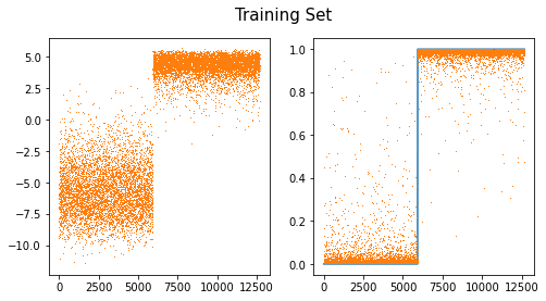

fig,ax = plt.subplots(1,2,figsize=(8,4))
ax[0].plot(net(XX).diff(axis=1).data,',',color="C1")
ax[1].plot(yy)
ax[1].plot(sftmax(net(XX))[:,1].data,',')
#ax[1].plot(sig(net(XX).diff(axis=1)).data,',')
fig.suptitle("Test Set",size=15)

Text(0.5, 0.98, 'Test Set')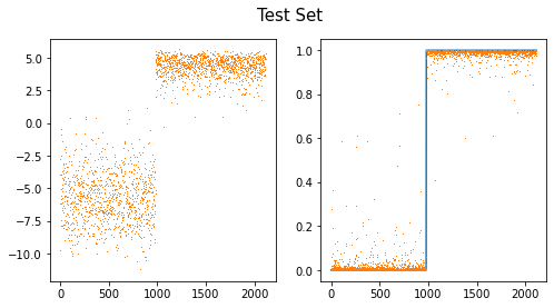

- note: softmax(u1,u2)=[sig(u1-u2), sig(u2-u1)]=[1-sig(u2-u1),sig(u2-u1)]

$\frac{1}{e^{u_{1}} + e^{u_{2}}} \to \frac{e^{u_{1} - u_{2}}}{e^{u_{1} - u_{2}} + e^{u_{2} - u_{2}}} \to \frac{e^{u_{1} - u_{2}}}{e^{u_{1} - u_{2}} + 1} \to s i g (u_{2} - u_{1})$

공부: 이진분류에서 소프트맥스 vs 시그모이드

- 이진분류문제 = “y=0 or y=1” 을 맞추는 문제 = 성공과 실패를 맞추는 문제 = 성공확률과 실패확률을 추정하는 문제

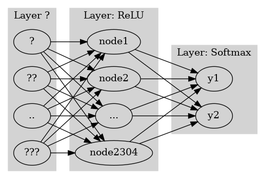
- softmax, sigmoid - softmax: (실패확률, 성공확률) 꼴로 결과가 나옴 // softmax는 실패확률과 성공확률을 둘다 추정한다. - sigmoid: (성공확률) 꼴로 결과가 나옴 // sigmoid는 성공확률만 추정한다.

- 그런데 “실패확률=1-성공확률” 이므로 사실상 둘은 같은걸 추정하는 셈이다. (성공확률만 추정하면 실패확률은 저절로 추정되니까)

- 아래는 사실상 같은 모형이다.

#collapse
gv('''
splines=line
subgraph cluster_1{
    style=filled;
    color=lightgrey;
    "?"
    "??"
    ".."
    "???"
    label = "Layer ?"
}
subgraph cluster_2{
    style=filled;
    color=lightgrey;
    "?" -> "node1"
    "??" -> "node1"
    ".." -> "node1"
    "???" -> "node1"
    
    "?" -> "node2"
    "??" -> "node2"
    ".." -> "node2"
    "???" -> "node2"
    
    "?" -> "..."
    "??" -> "..."
    ".." -> "..."
    "???" -> "..."
    
    "?" -> "node2304"
    "??" -> "node2304"
    ".." -> "node2304"
    "???" -> "node2304"

    label = "Layer: ReLU"
}
subgraph cluster_3{
    style=filled;
    color=lightgrey;
    "node1" -> "y1"
    "node2" -> "y1"
    "..." -> "y1"
    "node2304" -> "y1"
    
    "node1" -> "y2"
    "node2" -> "y2"
    "..." -> "y2"
    "node2304" -> "y2"    
    label = "Layer: Softmax"
}
''')

#collapse
gv('''
splines=line
subgraph cluster_1{
    style=filled;
    color=lightgrey;
    "?"
    "??"
    ".."
    "???"
    label = "Layer ?"
}
subgraph cluster_2{
    style=filled;
    color=lightgrey;
    "?" -> "node1"
    "??" -> "node1"
    ".." -> "node1"
    "???" -> "node1"
    
    "?" -> "node2"
    "??" -> "node2"
    ".." -> "node2"
    "???" -> "node2"
    
    "?" -> "..."
    "??" -> "..."
    ".." -> "..."
    "???" -> "..."
    
    "?" -> "node2304"
    "??" -> "node2304"
    ".." -> "node2304"
    "???" -> "node2304"

    label = "Layer: ReLU"
}
subgraph cluster_3{
    style=filled;
    color=lightgrey;
    "node1" -> "y"
    "node2" -> "y"
    "..." -> "y"
    "node2304" -> "y"
    label = "Layer: Sigmoid"
}
''')

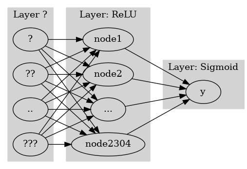
- 둘은 사실상 같은 효과를 주는 모형인데 학습할 파라메터는 sigmoid의 경우가 더 적다. $\to$ sigmoid를 사용하는 모형이 비용은 싸고(학습할 파라메터가 적음) 효과는 동일하다는 말 $\to$ 이진분류 한정해서는 softmax를 쓰지말고 sigmoid를 써야함. - softmax가 갑자기 너무 안좋아보이는데 sigmoid는 k개의 클래스로 확장이 불가능한 반면 softmax는 확장이 용이하다는 장점이 있음

소프트맥스 vs 시그모이드 정리

- 결론 1. 소프트맥스는 시그모이드의 확장이다. 2. 클래스의 수가 2개일 경우에는 (Sigmoid, BCEloss) 조합을 사용해야 하고 클래스의 수가 2개보다 클 경우에는 (Softmax, CrossEntropyLoss) 를 사용해야 한다.

- 그런데 사실.. 클래스의 수가 2개일 경우일때 (Softmax, CrossEntropyLoss)를 사용해도 그렇게 큰일나는것은 아니다. (흑백이미지를 칼라잉크로 출력하는 느낌)

참고

$y$	분포가정	마지막층의 활성화함수	손실함수
3.45, 4.43, … (연속형)	정규분포	None (or Identity)	MSE
0 or 1	이항분포 with $n = 1$ (=베르누이)	Sigmoid	BCE
[0,0,1], [0,1,0], [1,0,0]	다항분포 with $n = 1$	Softmax	Cross Entropy

fastai metric 사용

데이터준비

- download data

path = untar_data(URLs.MNIST)

- training set

X0 = torch.stack([torchvision.io.read_image(str(fname)) for fname in (path/'training/0').ls()])
X1 = torch.stack([torchvision.io.read_image(str(fname)) for fname in (path/'training/1').ls()])
X = torch.concat([X0,X1])/255
y = torch.tensor([0.0]*len(X0) + [1.0]*len(X1)).reshape(-1,1)

- test set

X0 = torch.stack([torchvision.io.read_image(str(fname)) for fname in (path/'testing/0').ls()])
X1 = torch.stack([torchvision.io.read_image(str(fname)) for fname in (path/'testing/1').ls()])
XX = torch.concat([X0,X1])/255
yy = torch.tensor([0.0]*len(X0) + [1.0]*len(X1)).reshape(-1,1)

X.shape,XX.shape,y.shape,yy.shape

(torch.Size([12665, 1, 28, 28]),
 torch.Size([2115, 1, 28, 28]),
 torch.Size([12665, 1]),
 torch.Size([2115, 1]))

사용자정의 메트릭이용

dls 만들기

ds1 = torch.utils.data.TensorDataset(X,y)
ds2 = torch.utils.data.TensorDataset(XX,yy)
dl1 = torch.utils.data.DataLoader(ds1,batch_size=1266) 
dl2 = torch.utils.data.DataLoader(ds2,batch_size=2115) 
dls = DataLoaders(dl1,dl2)

lrnr 생성

net = torch.nn.Sequential(
    torch.nn.Conv2d(1,16,(5,5)),
    torch.nn.ReLU(),
    torch.nn.MaxPool2d((2,2)),
    torch.nn.Flatten(),
    torch.nn.Linear(2304,1),
    torch.nn.Sigmoid()
)
loss_fn = torch.nn.BCELoss()

def acc(yhat,y) : 
    return ((yhat>0.5)==y).float().mean()

def err(yhat,y):
    return 1-((yhat>0.5)==y).float().mean()

lrnr = Learner(dls,net,loss_fn,metrics=[acc,err])

학습

lrnr.fit(10)

epoch	train_loss	valid_loss	acc	err	time
0	1.012566	0.676096	0.463357	0.536643	00:00
1	0.738655	0.477148	0.994799	0.005201	00:00
2	0.603908	0.335415	0.985816	0.014184	00:00
3	0.497049	0.183633	0.995745	0.004255	00:00
4	0.394664	0.097668	0.995745	0.004255	00:00
5	0.309929	0.056333	0.995745	0.004255	00:00
6	0.244836	0.037147	0.995745	0.004255	00:00
7	0.195441	0.027278	0.995745	0.004255	00:00
8	0.157570	0.021531	0.995745	0.004255	00:00
9	0.128163	0.017795	0.997163	0.002837	00:00

예측

생략

fastai지원 메트릭이용– 잘못된사용

dls 만들기

ds1 = torch.utils.data.TensorDataset(X,y)
ds2 = torch.utils.data.TensorDataset(XX,yy)
dl1 = torch.utils.data.DataLoader(ds1,batch_size=1266) 
dl2 = torch.utils.data.DataLoader(ds2,batch_size=2115) 
dls = DataLoaders(dl1,dl2)

lrnr 생성

net = torch.nn.Sequential(
    torch.nn.Conv2d(1,16,(5,5)),
    torch.nn.ReLU(),
    torch.nn.MaxPool2d((2,2)),
    torch.nn.Flatten(),
    torch.nn.Linear(2304,1),
    torch.nn.Sigmoid()
)
loss_fn = torch.nn.BCELoss()
lrnr = Learner(dls,net,loss_fn,metrics=[accuracy,error_rate])

accuracy??

Signature: accuracy(inp, targ, axis=-1)
Source:   
def accuracy(inp, targ, axis=-1):
    "Compute accuracy with `targ` when `pred` is bs * n_classes"
    pred,targ = flatten_check(inp.argmax(dim=axis), targ)
    return (pred == targ).float().mean()
File:      ~/anaconda3/envs/csy/lib/python3.8/site-packages/fastai/metrics.py
Type:      function

error_rate??

Signature: error_rate(inp, targ, axis=-1)
Source:   
def error_rate(inp, targ, axis=-1):
    "1 - `accuracy`"
    return 1 - accuracy(inp, targ, axis=axis)
File:      ~/anaconda3/envs/csy/lib/python3.8/site-packages/fastai/metrics.py
Type:      function

학습

lrnr.fit(10)

epoch	train_loss	valid_loss	accuracy	error_rate	time
0	0.971997	0.616424	0.463357	0.536643	00:00
1	0.671642	0.380434	0.463357	0.536643	00:00
2	0.525948	0.232161	0.463357	0.536643	00:00
3	0.414203	0.123899	0.463357	0.536643	00:00
4	0.322394	0.071857	0.463357	0.536643	00:00
5	0.252299	0.045784	0.463357	0.536643	00:00
6	0.199783	0.032276	0.463357	0.536643	00:00
7	0.160118	0.024500	0.463357	0.536643	00:00
8	0.129659	0.019576	0.463357	0.536643	00:00
9	0.105914	0.016207	0.463357	0.536643	00:00

이상하다..?

예측

lrnr.model.to("cpu")

Sequential(
  (0): Conv2d(1, 16, kernel_size=(5, 5), stride=(1, 1))
  (1): ReLU()
  (2): MaxPool2d(kernel_size=(2, 2), stride=(2, 2), padding=0, dilation=1, ceil_mode=False)
  (3): Flatten(start_dim=1, end_dim=-1)
  (4): Linear(in_features=2304, out_features=1, bias=True)
  (5): Sigmoid()
)

plt.plot(yy)
plt.plot(lrnr.model(XX).data,'.')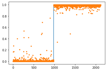

맞추는건 잘 맞추는데?

fastai지원 메트릭이용– 올바른 사용(1)

- 가정 - X의 형태는 (n,채널,픽셀,픽셀)로 가정한다. - y의 형태는 (n,) 벡터이다. 즉 $n \times 1$ 이 아니라 그냥 길이가 $n$ 인 벡터로 가정한다. - y의 각 원소는 0,1,2,3,… 와 같이 카테고리를 의미하는 숫자이어야 하며 이 숫자는 int형으로 저장되어야 한다. - loss function은 CrossEntropyLoss()를 쓴다고 가정한다. (따라서 네트워크의 최종레이어는 torch.nn.Linear(?,클래스의수) 꼴이 되어야 한다.)

dls 만들기

지원하는 함수로 바꿔주기

y.to(torch.int64).reshape(-1),yy.to(torch.int64).reshape(-1)

(tensor([0, 0, 0,  ..., 1, 1, 1]), tensor([0, 0, 0,  ..., 1, 1, 1]))

ds1 = torch.utils.data.TensorDataset(X,y.to(torch.int64).reshape(-1))
ds2 = torch.utils.data.TensorDataset(XX,yy.to(torch.int64).reshape(-1))
dl1 = torch.utils.data.DataLoader(ds1,batch_size=1266) 
dl2 = torch.utils.data.DataLoader(ds2,batch_size=2115) 
dls = DataLoaders(dl1,dl2)

lrnr 생성

net = torch.nn.Sequential(
    torch.nn.Conv2d(1,16,(5,5)),
    torch.nn.ReLU(),
    torch.nn.MaxPool2d((2,2)),
    torch.nn.Flatten(),
    torch.nn.Linear(2304,2),
)
loss_fn = torch.nn.CrossEntropyLoss()
lrnr = Learner(dls,net,loss_fn,metrics=[accuracy,error_rate])

학습

lrnr.fit(10)

epoch	train_loss	valid_loss	accuracy	error_rate	time
0	1.038122	0.539247	0.463357	0.536643	00:00
1	0.621439	0.261176	0.977778	0.022222	00:00
2	0.451623	0.118811	0.989125	0.010875	00:00
3	0.333172	0.059299	0.995272	0.004728	00:00
4	0.250918	0.037678	0.996217	0.003783	00:00
5	0.193416	0.026810	0.996217	0.003783	00:00
6	0.152078	0.020631	0.996217	0.003783	00:00
7	0.121511	0.016605	0.996690	0.003310	00:00
8	0.098301	0.013718	0.997636	0.002364	00:00
9	0.080287	0.011546	0.998109	0.001891	00:00

fastai지원 메트릭이용– 올바른 사용(2)

- 가정 - X의 형태는 (n,채널,픽셀,픽셀)로 가정한다. - y의 형태는 (n,클래스의수)로 가정한다. 즉 y가 one_hot 인코딩된 형태로 가정한다. - y의 각 원소는 0 혹은 1이다. - loss function은 CrossEntropyLoss()를 쓴다고 가정한다. (따라서 네트워크의 최종레이어는 torch.nn.Linear(?,클래스의수) 꼴이 되어야 한다.)

dls 만들기

y_onehot = torch.tensor(list(map(lambda x: [1.0,0.0] if x==0 else [0.0,1.0], y)))
yy_onehot = torch.tensor(list(map(lambda x: [1.0,0.0] if x==0 else [0.0,1.0], yy)))
# y_onehot = torch.nn.functional.one_hot(y.reshape(-1).to(torch.int64)).to(torch.float32)
# yy_onehot = torch.nn.functional.one_hot(yy.reshape(-1).to(torch.int64)).to(torch.float32)

ds1 = torch.utils.data.TensorDataset(X,y_onehot)
ds2 = torch.utils.data.TensorDataset(XX,yy_onehot)
dl1 = torch.utils.data.DataLoader(ds1,batch_size=1266) 
dl2 = torch.utils.data.DataLoader(ds2,batch_size=2115) 
dls = DataLoaders(dl1,dl2)

lrnr 생성

net = torch.nn.Sequential(
    torch.nn.Conv2d(1,16,(5,5)),
    torch.nn.ReLU(),
    torch.nn.MaxPool2d((2,2)),
    torch.nn.Flatten(),
    torch.nn.Linear(2304,2),
    #torch.nn.Softmax()
)
loss_fn = torch.nn.CrossEntropyLoss() 
lrnr = Learner(dls,net,loss_fn,metrics=[accuracy_multi])

accuracy_multi

학습

lrnr.fit(10)

epoch	train_loss	valid_loss	accuracy_multi	time
0	1.038750	0.569555	0.463357	00:00
1	0.640057	0.285553	0.977778	00:00
2	0.469265	0.137582	0.987943	00:00
3	0.348698	0.064898	0.995035	00:00
4	0.262547	0.038338	0.996217	00:00
5	0.201805	0.025988	0.996690	00:00
6	0.158089	0.019443	0.996927	00:00
7	0.125811	0.015470	0.997163	00:00
8	0.101381	0.012772	0.998109	00:00
9	0.082515	0.010802	0.998582	00:00